Custom visualizations with Vega

Vega and Vega-Lite are grammars for creating custom visualizations. You write a JSON (or HJSON) specification that defines the data, transforms, and visual marks. Vega-Lite is a good starting point if you are new to both grammars, but they are not compatible.

Add a Vega panel on a dashboard to use these grammars with Kibana filters, the time range, and other Kibana extensions. You can set the panel's data source to:

• Elasticsearch, using:
  • An ES|QL query (recommended). One query string replaces nested Query DSL aggregations and format paths. See Writing ES|QL queries in Vega.
  • An Elasticsearch Query DSL search. Use this approach when ES|QL is unavailable, or when you already have a Query DSL request you want to reuse.
• Elastic Map Service vector shapes
• A file at an external URL, using Vega's native url data source
• Static values written directly into the spec, using Vega's native inline data

×

For most charts, start with Visualizations, using either point-and-click or an ES|QL query. Use Maps for geographic data.

Choose Vega when you need full control of the specification, for example:

• Chart types that other editors do not support, such as scatter charts, sankey charts, or a custom visual theme
• Aggregations that use nested or parent/child mapping
• Aggregations without a data view
• Queries that use custom time filters
• Complex calculations
• Data extracted from _source instead of aggregations
• Multiple data sources in one panel

Vega and Vega-Lite do not support tables, and can’t run queries conditionally.

These tutorials walk you through building Vega and Vega-Lite panels on a dashboard: define a data source, shape the chart, and optionally update Kibana filters from the visualization.

As you edit the specs, work in small steps and save often. Small changes can cause unexpected results. Specs can use HJSON, which allows optional quotes and commas, comments, and multiline strings.

Learn how to query your data with ES|QL from Vega-Lite and display the results in a line chart.

1. Install the sample web logs data set.
2. Go to Dashboards.
3. On the Dashboards page, select Create dashboard.

1. Select Add in the application menu.

2. Select Vega or Custom visualization: you might see either name depending on your Kibana version.

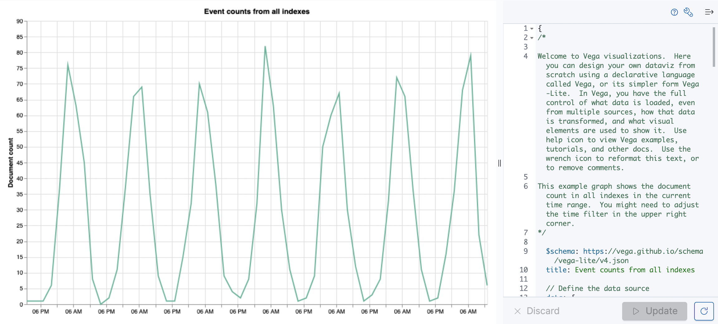
   A pre-populated line chart displays the total number of documents.

3. Set the time filter to a range that includes the sample data. Sample data timestamps are relative to when you installed the data set, so Last 7 days works if you just installed it.

4. Replace the entire Vega-Lite spec with the following, then select Update:

{
  "$schema": "https://vega.github.io/schema/vega-lite/v6.json",
  "title": "Event counts over time",
  "data": {
    "url": {
      "%type%": "esql",
      "%context%": true,
      "%timefield%": "@timestamp",
      "query": "FROM kibana_sample_data_logs | WHERE @timestamp >= ?_tstart AND @timestamp <= ?_tend | STATS doc_count=COUNT() BY key=DATE_TRUNC(2 hour, @timestamp) | SORT key"
    }
  },
  "mark": "line",
  "encoding": {
    "x": {
      "field": "key",
      "type": "temporal",
      "axis": {"title": false}
    },
    "y": {
      "field": "doc_count",
      "type": "quantitative",
      "axis": {"title": "Document count"}
    }
  }
}
		

1. Tells Kibana to run the query as ES|QL.
2. Applies the dashboard filters to the query.
3. Enables the ?_tstart and ?_tend named parameters so the query uses the dashboard time range.
4. The ES|QL query. Kibana converts the columnar response into the row-based format that Vega expects.

The chart shows event counts over time from kibana_sample_data_logs. For the full list of ES|QL url parameters, see Writing ES|QL queries in Vega.

To continue with interactive filtering and Query DSL examples, see Create a stacked area chart from an Elasticsearch search query and Update Kibana filters from Vega.

Learn how to query Elasticsearch with Query DSL from Vega-Lite, displaying the results in a stacked area chart.

If you completed the ES|QL tutorial, create a new dashboard (or clear the editor) before you continue.

1. Install the eCommerce sample data set.

2. Go to Dashboards.

3. On the Dashboards page, select Create dashboard.

4. Select Add (or Add panel in earlier versions) in the application menu, then select Vega or Custom visualization: you might see either name depending on your Kibana version.

   A pre-populated line chart displays the total number of documents.

5. Set the time filter to a range that includes the sample data. Sample data timestamps are relative to when you installed the data set, so Last 7 days works if you just installed it.

1. In the Vega-Lite spec, replace index: _all with the following, then click Update:

index: kibana_sample_data_ecommerce
		

A flat line appears with zero results.

To add the data fields from the kibana_sample_data_ecommerce data view, replace the following, then click Update:

• %timefield%: @timestamp with %timefield%: order_date
• field: @timestamp with field: order_date

To create the stacked area chart, add the aggregations.

To check your work, open and use the Console on a separate browser tab.

1. Open Kibana on a new tab.
2. Go to the Developer tools page using the navigation menu or the global search field.
3. On the Console editor, enter the aggregation, then click Click to send request:

POST kibana_sample_data_ecommerce/_search
{
  "query": {
    "range": {
      "order_date": {
        "gte": "now-7d"
      }
    }
  },
  "aggs": {
    "time_buckets": {
      "date_histogram": {
        "field": "order_date",
        "fixed_interval": "1d",
        "extended_bounds": {
          "min": "now-7d"
        },
        "min_doc_count": 0
      }
    }
  },
  "size": 0
}
		

Add the terms aggregation, then click Click to send request:

POST kibana_sample_data_ecommerce/_search
{
  "query": {
    "range": {
      "order_date": {
        "gte": "now-7d"
      }
    }
  },
  "aggs": {
    "categories": {
      "terms": { "field": "category.keyword" },
      "aggs": {
        "time_buckets": {
          "date_histogram": {
            "field": "order_date",
            "fixed_interval": "1d",
            "extended_bounds": {
              "min": "now-7d"
            },
            "min_doc_count": 0
          }
        }
      }
    }
  },
  "size": 0
}
		

The response format is different from the first aggregation query:

{
  "aggregations" : {
    "categories" : {
      "doc_count_error_upper_bound" : 0,
      "sum_other_doc_count" : 0,
      "buckets" : [{
        "key" : "Men's Clothing",
        "doc_count" : 1661,
        "time_buckets" : {
          "buckets" : [{
            "key_as_string" : "2020-06-30T00:00:00.000Z",
            "key" : 1593475200000,
            "doc_count" : 19
          }, {
            "key_as_string" : "2020-07-01T00:00:00.000Z",
            "key" : 1593561600000,
            "doc_count" : 71
          }]
        }
      }]
    }
  }
}
		

In the Vega-Lite spec, enter the aggregations, then click Update:

data: {
  url: {
    %context%: true
    %timefield%: order_date
    index: kibana_sample_data_ecommerce
    body: {
      aggs: {
        categories: {
          terms: { field: "category.keyword" }
          aggs: {
            time_buckets: {
              date_histogram: {
                field: order_date
                interval: {%autointerval%: true}
                extended_bounds: {
                  min: {%timefilter%: "min"}
                  max: {%timefilter%: "max"}
                }
                min_doc_count: 0
              }
            }
          }
        }
      }
      size: 0
    }
  }
  format: {property: "aggregations.categories.buckets" }
}
		

For information about the queries, refer to reference for writing Elasticsearch queries in Vega.

To generate the data, Vega-Lite uses the source_0 and data_0. source_0 contains the results from the Elasticsearch query, and data_0 contains the visually encoded results that are shown on the chart. To debug the warning, compare source_0 and data_0.

1. In the toolbar, click Inspect.

2. From the View dropdown, select Vega debug.

3. From the dropdown, select source_0.

   
   ×

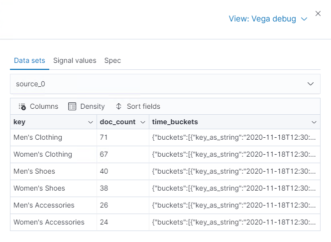
4. To compare to the visually encoded data, select data_0 from the dropdown.

   
   ×

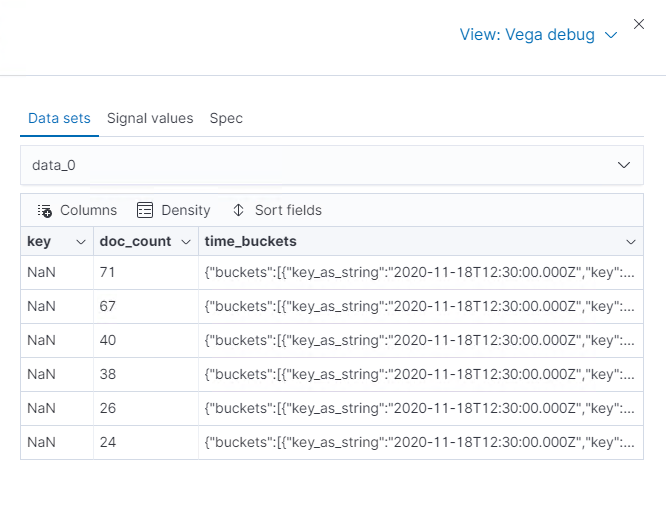
   key is unable to convert because the property is category (Men's Clothing, Women's Clothing, etc.) instead of a timestamp.

In the Vega-Lite spec, add the encoding block:

encoding: {
  x: {
    field: time_buckets.buckets.key
    type: temporal
    axis: { title: null }
  }
  y: {
    field: time_buckets.buckets.doc_count
    type: quantitative
    axis: { title: "Document count" }
  }
}
		

1. Click Inspect, then select Vega Debug from the View dropdown.

2. From the dropdown, select data_0.

   
   ×

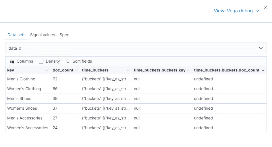
Vega-Lite is unable to extract the time_buckets.buckets inner array.

In Kibana 7.9 and later, use the Vega-Lite flatten transformation to extract the time_buckets.buckets inner array.

If you are using Kibana 7.8 and earlier, the flatten transformation is available only in Vega.

In the Vega-Lite spec, add a transform block, then click Update:

transform: [{
  flatten: ["time_buckets.buckets"]
}]
		

1. Click Inspect, then select Vega Debug from the View dropdown.

2. From the dropdown, select data_0.

   
   ×

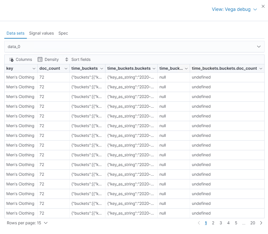
   Vega-Lite displays undefined values because there are duplicate names.

3. To resolve the duplicate names, add the transform and encoding blocks, then click Update:

transform: [{
  flatten: ["time_buckets.buckets"],
  as: ["buckets"]
}]

mark: area

encoding: {
  x: {
    field: buckets.key
    type: temporal
    axis: { title: null }
  }
  y: {
    field: buckets.doc_count
    type: quantitative
    axis: { title: "Document count" }
  }
  color: {
    field: key
    type: nominal
  }
}
		

With the Vega-Lite spec, you can add hover states and tooltips to the stacked area chart with the selection block.

In the Vega-Lite spec, add the encoding block, then click Update:

encoding: {
  tooltip: [{
    field: buckets.key
    type: temporal
    title: "Date"
  }, {
    field: key
    type: nominal
    title: "Category"
  }, {
    field: buckets.doc_count
    type: quantitative
    title: "Count"
  }]
}
		

When you hover over the area series on the stacked area chart, a multi-line tooltip appears, but is unable to indicate the nearest point. To indicate the nearest point, add a second layer.

Add composite marks, then click Update:

layer: [{
  mark: area
}, {
  mark: point
}]
		

The points are unable to stack and align with the stacked area chart.

Change the y encoding:

y: {
  field: buckets.doc_count
  type: quantitative
  axis: { title: "Document count" }
  stack: true
}
		

Add a selection block inside mark: point:

layer: [{
  mark: area
}, {
  mark: point

  selection: {
    pointhover: {
      type: single
      on: mouseover
      clear: mouseout
      empty: none
      fields: ["buckets.key", "key"]
      nearest: true
    }
  }

  encoding: {
    size: {
      condition: {
        selection: pointhover
        value: 100
      }
      value: 5
    }
    fill: {
      condition: {
        selection: pointhover
        value: white
      }
    }
  }
}]
		

Move your cursor around the stacked area chart. The points are able to indicate the nearest point.

×

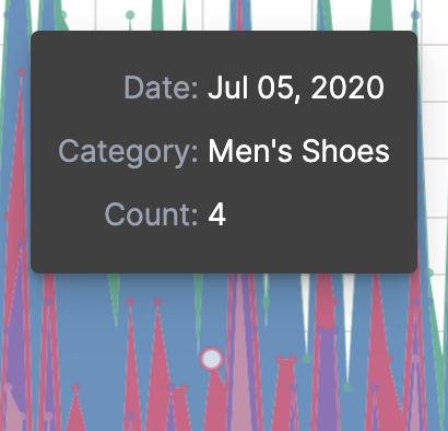
The selection is controlled by a signal. To view the signal, click Inspect in the toolbar.

{
  $schema: https://vega.github.io/schema/vega-lite/v4.json
  title: Event counts from ecommerce
  data: {
    url: {
      %context%: true
      %timefield%: order_date
      index: kibana_sample_data_ecommerce
      body: {
        aggs: {
          categories: {
            terms: { field: "category.keyword" }
            aggs: {
              time_buckets: {
                date_histogram: {
                  field: order_date
                  interval: {%autointerval%: true}
                  extended_bounds: {
                    min: {%timefilter%: "min"}
                    max: {%timefilter%: "max"}
                  }
                  min_doc_count: 0
                }
              }
            }
          }
        }
        size: 0
      }
    }
    format: {property: "aggregations.categories.buckets" }
  }

  transform: [{
    flatten: ["time_buckets.buckets"]
    as: ["buckets"]
  }]

  encoding: {
    x: {
      field: buckets.key
      type: temporal
      axis: { title: null }
    }
    y: {
      field: buckets.doc_count
      type: quantitative
      axis: { title: "Document count" }
      stack: true
    }
    color: {
      field: key
      type: nominal
      title: "Category"
    }
    tooltip: [{
      field: buckets.key
      type: temporal
      title: "Date"
    }, {
      field: key
      type: nominal
      title: "Category"
    }, {
      field: buckets.doc_count
      type: quantitative
      title: "Count"
    }]
  }

  layer: [{
    mark: area
  }, {
    mark: point

    selection: {
      pointhover: {
        type: single
        on: mouseover
        clear: mouseout
        empty: none
        fields: ["buckets.key", "key"]
        nearest: true
      }
    }

    encoding: {
      size: {
        condition: {
          selection: pointhover
          value: 100
        }
        value: 5
      }
      fill: {
        condition: {
          selection: pointhover
          value: white
        }
      }
    }
  }]
}
		

To build an area chart using an Elasticsearch search query, edit the Vega spec, then add click and drag handlers to update the Kibana filters.

In the Vega spec, enter the following, then click Update:

{
  $schema: "https://vega.github.io/schema/vega/v5.json"
  data: [{
    name: source_0
  }]

  scales: [{
    name: x
    type: time
    range: width
  }, {
    name: y
    type: linear
    range: height
  }]

  axes: [{
    orient: bottom
    scale: x
  }, {
    orient: left
    scale: y
  }]

  marks: [
    {
      type: area
      from: {
        data: source_0
      }
      encode: {
        update: {
        }
      }
    }
  ]
}
		

Add the Elasticsearch search query with the data block, then click Update:

data: [
  {
    name: source_0
    url: {
      %context%: true
      %timefield%: order_date
      index: kibana_sample_data_ecommerce
      body: {
        aggs: {
          time_buckets: {
            date_histogram: {
              field: order_date
              fixed_interval: "3h"
              extended_bounds: {
                min: {%timefilter%: "min"}
                max: {%timefilter%: "max"}
              }
              min_doc_count: 0
            }
          }
        }
        size: 0
      }
    }
    format: { property: "aggregations.time_buckets.buckets" }
  }
]
		

Display labels for the x- and y-axes.

In the Vega spec, add the scales block, then click Update:

scales: [{
  name: x
  type: time
  range: width
  domain: {
    data: source_0
    field: key
  }
}, {
  name: y
  type: linear
  range: height
  domain: {
    data: source_0
    field: doc_count
  }
}]
		

Add the key and doc_count fields as the X- and Y-axis values, then click Update:

marks: [
  {
    type: area
    from: {
      data: source_0
    }
    encode: {
      update: {
        x: {
          scale: x
          field: key
        }
        y: {
          scale: y
          value: 0
        }
        y2: {
          scale: y
          field: doc_count
        }
      }
    }
  }
]
		

×

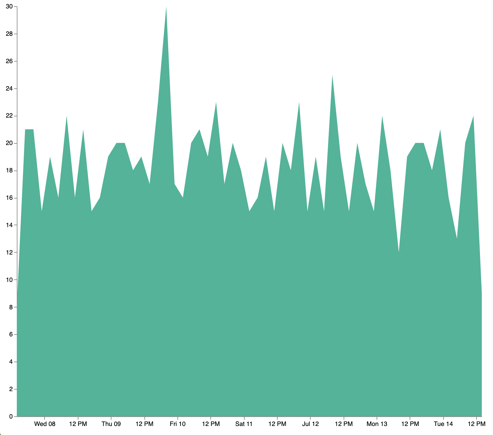
Show the clickable points on the area chart to filter for a specific date.

In the Vega spec, add to the marks block, then click Update:

{
  name: point
  type: symbol
  style: ["point"]
  from: {
    data: source_0
  }
  encode: {
    update: {
      x: {
        scale: x
        field: key
      }
      y: {
        scale: y
        field: doc_count
      }
      size: {
        value: 100
      }
      fill: {
        value: black
      }
    }
  }
}
		

To make the points clickable, create a Vega signal. You can access the clicked datum in the expression used to update.

In the Vega spec, add a signals block to specify that the cursor clicks add a time filter with the three hour interval, then click Update:

signals: [
  {
    name: point_click
    on: [{
      events: {
        source: scope
        type: click
        markname: point
      }
      update: '''kibanaSetTimeFilter(datum.key, datum.key + 3 * 60 * 60 * 1000)'''
    }]
  }
]
		

The event uses the kibanaSetTimeFilter custom function to generate a filter that applies to the entire dashboard on a click.

To make the area chart interactive, locate the marks block, then update the point and add cursor: { value: "pointer" } to encoding:

{
  name: point
  type: symbol
  style: ["point"]
  from: {
    data: source_0
  }
  encode: {
    update: {
      ...
      cursor: { value: "pointer" }
    }
  }
}
		

To allow users to filter based on a time range, add a drag interaction, which requires additional signals and a rectangle overlay.

×

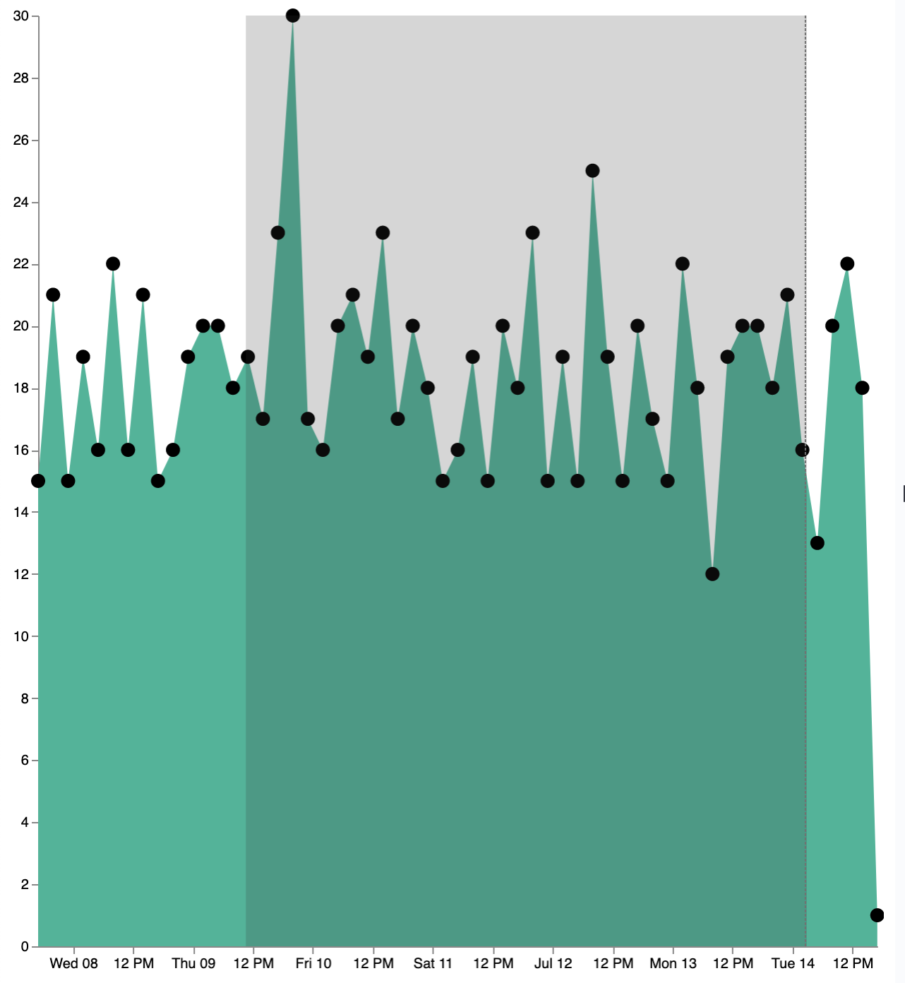
In the Vega spec, add a signal to track the X position of the cursor:

{
  name: currentX
  value: -1
  on: [{
    events: {
      type: mousemove
      source: view
    },
    update: "clamp(x(), 0, width)"
  }, {
    events: {
      type: mouseout
      source: view
    }
    update: "-1"
  }]
}
		

To indicate the current cursor position, add a mark block:

{
  type: rule
  interactive: false
  encode: {
    update: {
      y: {value: 0}
      y2: {signal: "height"}
      stroke: {value: "gray"}
      strokeDash: {
        value: [2, 1]
      }
      x: {signal: "max(currentX,0)"}
      defined: {signal: "currentX > 0"}
    }
  }
}
		

To track the selected time range, add a signal that updates until the user releases their cursor or presses Return:

{
  name: selected
  value: [0, 0]
  on: [{
    events: {
      type: mousedown
      source: view
    }
    update: "[clamp(x(), 0, width), clamp(x(), 0, width)]"
  }, {
    events: {
      type: mousemove
      source: window
      consume: true
      between: [{
        type: mousedown
        source: view
      }, {
        merge: [{
          type: mouseup
          source: window
        }, {
          type: keydown
          source: window
          filter: "event.key === 'Escape'"
        }]
      }]
    }
    update: "[selected[0], clamp(x(), 0, width)]"
  }, {
    events: {
      type: keydown
      source: window
      filter: "event.key === 'Escape'"
    }
    update: "[0, 0]"
  }]
}
		

There is a signal that tracks the time range from the user.

To indicate the range visually, add a mark that only appears conditionally:

{
  type: rect
  name: selectedRect
  encode: {
    update: {
      height: {signal: "height"}
      fill: {value: "#333"}
      fillOpacity: {value: 0.2}
      x: {signal: "selected[0]"}
      x2: {signal: "selected[1]"}
      defined: {signal: "selected[0] !== selected[1]"}
    }
  }
}
		

Add a signal that updates the Kibana time filter when the cursor is released while dragging:

{
  name: applyTimeFilter
  value: null
  on: [{
    events: {
      type: mouseup
      source: view
    }
    update: '''selected[0] !== selected[1] ? kibanaSetTimeFilter(
           invert('x',selected[0]),
           invert('x',selected[1])) : null'''
  }]
}
		

{
  $schema: "https://vega.github.io/schema/vega/v5.json"
  data: [
    {
      name: source_0
      url: {
        %context%: true
        %timefield%: order_date
        index: kibana_sample_data_ecommerce
        body: {
          aggs: {
            time_buckets: {
              date_histogram: {
                field: order_date
                fixed_interval: "3h"
                extended_bounds: {
                  min: {%timefilter%: "min"}
                  max: {%timefilter%: "max"}
                }
                min_doc_count: 0
              }
            }
          }
          size: 0
        }
      }
      format: { property: "aggregations.time_buckets.buckets" }
    }
  ]

  scales: [{
    name: x
    type: time
    range: width
    domain: {
      data: source_0
      field: key
    }
  }, {
    name: y
    type: linear
    range: height
    domain: {
      data: source_0
      field: doc_count
    }
  }]

  axes: [{
    orient: bottom
    scale: x
  }, {
    orient: left
    scale: y
  }]

  marks: [
    {
      type: area
      from: {
        data: source_0
      }
      encode: {
        update: {
          x: {
            scale: x
            field: key
          }
          y: {
            scale: y
            value: 0
          }
          y2: {
            scale: y
            field: doc_count
          }
        }
      }
    },
    {
      name: point
      type: symbol
      style: ["point"]
      from: {
        data: source_0
      }
      encode: {
        update: {
          x: {
            scale: x
            field: key
          }
          y: {
            scale: y
            field: doc_count
          }
          size: {
            value: 100
          }
          fill: {
            value: black
          }
          cursor: { value: "pointer" }
        }
      }
    },
    {
      type: rule
      interactive: false
      encode: {
        update: {
          y: {value: 0}
          y2: {signal: "height"}
          stroke: {value: "gray"}
          strokeDash: {
            value: [2, 1]
          }
          x: {signal: "max(currentX,0)"}
          defined: {signal: "currentX > 0"}
        }
      }
    },
    {
      type: rect
      name: selectedRect
      encode: {
        update: {
          height: {signal: "height"}
          fill: {value: "#333"}
          fillOpacity: {value: 0.2}
          x: {signal: "selected[0]"}
          x2: {signal: "selected[1]"}
          defined: {signal: "selected[0] !== selected[1]"}
        }
      }
    }
  ]

  signals: [
    {
      name: point_click
      on: [{
        events: {
          source: scope
          type: click
          markname: point
        }
        update: '''kibanaSetTimeFilter(datum.key, datum.key + 3 * 60 * 60 * 1000)'''
      }]
    }
    {
      name: currentX
      value: -1
      on: [{
        events: {
          type: mousemove
          source: view
        },
        update: "clamp(x(), 0, width)"
      }, {
        events: {
          type: mouseout
          source: view
        }
        update: "-1"
      }]
    }
    {
      name: selected
      value: [0, 0]
      on: [{
        events: {
          type: mousedown
          source: view
        }
        update: "[clamp(x(), 0, width), clamp(x(), 0, width)]"
      }, {
        events: {
          type: mousemove
          source: window
          consume: true
          between: [{
            type: mousedown
            source: view
          }, {
            merge: [{
              type: mouseup
              source: window
            }, {
              type: keydown
              source: window
              filter: "event.key === 'Escape'"
            }]
          }]
        }
        update: "[selected[0], clamp(x(), 0, width)]"
      }, {
        events: {
          type: keydown
          source: window
          filter: "event.key === 'Escape'"
        }
        update: "[0, 0]"
      }]
    }
    {
      name: applyTimeFilter
      value: null
      on: [{
        events: {
          type: mouseup
          source: view
        }
        update: '''selected[0] !== selected[1] ? kibanaSetTimeFilter(
               invert('x',selected[0]),
               invert('x',selected[1])) : null'''
      }]
    }
  ]
}
		

Learn more about Kibana extension, additional Vega resources, and examples.

Kibana has extended Vega and Vega-Lite with extensions that support:

• Automatic sizing
• Default theme to match Kibana
• Writing ES|QL queries using the time range and filters from dashboards
• Writing Elasticsearch queries using the time range and filters from dashboards
• Using the Elastic Map Service in Vega maps
• Additional tooltip styling
• Advanced setting to enable URL loading from any domain
• Debugging support using the Kibana inspector
• (Vega only) Expression functions which can update the time range and dashboard filters

Most users will want their Vega visualizations to take the full available space, so unlike Vega examples, width and height are not required parameters in Kibana because your spec will be merged with the default Kibana settings in most cases:

autosize: {
  type: fit
  contains: padding
}
width: container
height: container
		

These default settings are not applied if:

• Your spec uses type=map
• Your spec is Vega-Lite and contains a facet, row, column, repeat, or concat operator. In these cases, providing width and height will affect the child size.

To set the width or height manually, set autosize: none and provide the exact pixel sizes, including padding for the title, legend and axes.

autosize: none
width: 600
height: 200
padding: {
  top: 20
  bottom: 20
  left: 55
  right: 150
}
		

To learn more, read about Vega autosize and Vega-Lite autosize.

Kibana registers a default Vega color scheme with the id elastic, and sets a default color for each mark type. Override it by providing a different stroke, fill, or color (Vega-Lite) value.

Prefer Writing ES|QL queries in Vega when you can use ES|QL. Use the Query DSL approach in this section when ES|QL is unavailable, or when you already have a Query DSL request you want to reuse.

Kibana extends the Vega data elements with support for direct Elasticsearch queries specified as url.

Kibana is unable to support dynamically loaded data, which would otherwise work in Vega. All data is fetched before it’s passed to the Vega renderer.

To define an Elasticsearch query in Vega, set the url to an object. Kibana parses the object looking for special tokens that allow your query to integrate with Kibana.

Tokens include the following:

• %context%: true: Set at the top level, and replaces the query section with filters from dashboard
• %timefield%: <name>: Set at the top level, integrates the query with the dashboard time filter
• {%timefilter%: true}: Replaced by an Elasticsearch range query with upper and lower bounds
• {%timefilter%: "min" | "max"}: Replaced only by the upper or lower bounds
• {%timefilter: true, shift: -1, unit: 'hour'}: Generates a time range query one hour in the past
• {%autointerval%: true}: Replaced by the string which contains the automatic Kibana time interval, such as 1h
• {%autointerval%: 10}: Replaced by a string which is approximately dividing the time into 10 ranges, allowing you to influence the automatic interval
• "%dashboard_context-must_clause%": String replaced by object containing filters
• "%dashboard_context-filter_clause%": String replaced by an object containing filters
• "%dashboard_context-must_not_clause%": String replaced by an object containing filters

For example, the following query counts the number of documents in a specific index:

// An object instead of a string for the URL value
// is treated as a context-aware Elasticsearch query.
url: {
  // Specify the time filter.
  %timefield%: @timestamp
  // Apply dashboard context filters when set
  %context%: true

  // Which indexes to search
  index: kibana_sample_data_logs
  // The body element may contain "aggs" and "query" keys
  body: {
    aggs: {
      time_buckets: {
        date_histogram: {
          // Use date histogram aggregation on @timestamp field
          field: @timestamp
          // interval value will depend on the time filter
          // Use an integer to set approximate bucket count
          interval: { %autointerval%: true }
          // Make sure we get an entire range, even if it has no data
          extended_bounds: {
            min: { %timefilter%: "min" }
            max: { %timefilter%: "max" }
          }
          // Use this for linear (e.g. line, area) graphs
          // Without it, empty buckets will not show up
          min_doc_count: 0
        }
      }
    }
    // Speed up the response by only including aggregation results
    size: 0
  }
}
		

1. @timestamp — Filters the time range and breaks it into histogram buckets.

The full result includes the following structure:

{
  "aggregations": {
    "time_buckets": {
      "buckets": [{
          "key_as_string": "2015-11-30T22:00:00.000Z",
          "key": 1448920800000,<1>
          "doc_count": 28
        }, {
          "key_as_string": "2015-11-30T23:00:00.000Z",
          "key": 1448924400000,
          "doc_count": 330
        }, ...
		

1. "key" — The unix timestamp you can use without conversions by the Vega date expressions.

For most visualizations, you only need the list of bucket values. To focus on only the data you need, use format: {property: "aggregations.time_buckets.buckets"}.

Specify a query with individual range and dashboard context. The query is equivalent to "%context%": true, "%timefield%": "@timestamp", except that the time range is shifted back by 10 minutes:

{
  body: {
    query: {
      bool: {
        must: [
          // This string will be replaced
          // with the auto-generated "MUST" clause
          "%dashboard_context-must_clause%"
          {
            range: {
              // apply timefilter (upper right corner)
              // to the @timestamp variable
              @timestamp: {
                // "%timefilter%" will be replaced with
                // the current values of the time filter
                // (from the upper right corner)
                "%timefilter%": true
                // Only work with %timefilter%
                // Shift current timefilter by 10 units back
                shift: 10
                // week, day (default), hour, minute, second
                unit: minute
              }
            }
          }
        ]
        must_not: [
          // This string will be replaced with
          // the auto-generated "MUST-NOT" clause
          "%dashboard_context-must_not_clause%"
        ]
        filter: [
          // This string will be replaced
          // with the auto-generated "FILTER" clause
          "%dashboard_context-filter_clause%"
        ]
      }
    }
  }
}
		

The "%timefilter%" can also be used to specify a single min or max value. The date_histogram’s extended_bounds can be set with two values - min and max. Instead of hardcoding a value, you may use "min": {"%timefilter%": "min"}, which will be replaced with the beginning of the current time range. The shift and unit values are also supported. The "interval" can also be set dynamically, depending on the currently picked range: "interval": {"%autointerval%": 10} will try to get about 10-15 data points (buckets).

To get started with a worked example, see Create a line chart from an ES|QL query. For Query DSL instead, see Writing Elasticsearch queries in Vega.

To use an ES|QL query as a data source, set "%type%" to "esql" in the url object and provide your query in the "query" parameter. ES|QL queries work in both Vega and Vega-Lite visualizations.

{
  "data": [
    {
      "name": "my_data",
      "url": {
        "%type%": "esql",
        "query": "FROM kibana_sample_data_logs | STATS count=COUNT()"
      }
    }
  ]
}
		

The url object supports the following parameters:

The response is converted from the ES|QL columnar format into the row-based format that Vega expects, with one object per row keyed by column name.

The following example creates a metric that counts documents over time, using the dashboard filters and time range through "%context%", "%timefield%", and the ?_tstart and ?_tend parameters. To try it, install the sample web logs data set, open a new custom visualization on a dashboard, and paste the spec:

{
  "$schema": "https://vega.github.io/schema/vega-lite/v6.json",
  "title": "Event counts over time",
  "data": {
    "url": {
      "%type%": "esql",
      "%context%": true,
      "%timefield%": "@timestamp",
      "query": "FROM kibana_sample_data_logs | WHERE @timestamp >= ?_tstart AND @timestamp <= ?_tend | STATS doc_count=COUNT() BY key=DATE_TRUNC(2 hour, @timestamp) | SORT key"
    }
  },
  "mark": "line",
  "encoding": {
    "x": {
      "field": "key",
      "type": "temporal",
      "axis": {"title": false}
    },
    "y": {
      "field": "doc_count",
      "type": "quantitative",
      "axis": {"title": "Document count"}
    }
  }
}
		

Vega and Vega-Lite panels that use an ES|QL data source are subject to the Fast mode dashboard option. When this option is active on a dashboard, these panels return faster, estimated results for STATS aggregations.

Access the Elastic Map Service files using the same mechanism:

url: {
  // "type" defaults to "elasticsearch" otherwise
  %type%: emsfile
  // Name of the file, exactly as in https://maps.elastic.co
  name: World Countries
}
// The result is either a topojson file or a geojson file.
// Refer to the Default format for the file at https://maps.elastic.co
// Get its features to use this data source with the "shape" marks
// https://vega.github.io/vega/docs/marks/shape/
// For a topojson file use
format: {type: "topojson", feature: "data"}

// For a geojson file use
format: {property: "features"}
		

Kibana has installed the Vega tooltip plugin, so tooltips can be defined in the ways documented there. Beyond that, Kibana also supports a configuration option for changing the tooltip position and padding:

{
  config: {
    kibana: {
      tooltips: {
        position: 'top',
        padding: 15,
        textTruncate: true,
      }
    }
  }
}
		

Vega can load data from any URL. To enable, set vis_type_vega.enableExternalUrls: true in kibana.yml, then restart Kibana.

The files that the external URLs load must allow CORS. The remote URL must include Access-Control-Allow-Origin, which allows requests from the Kibana URL.

You can make the current time range part of the external as a millisecond timestamp by using the placeholders %timefilter_min% and %timefilter_max%, e.g. http://example.com?min=%timefilter_min%.

Use the contextual Inspect tool to gain insights into different elements.

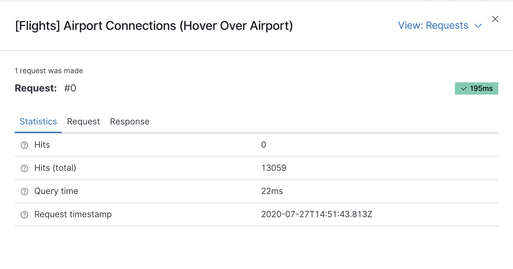
Vega uses the Elasticsearch search API to get documents and aggregation results from Elasticsearch. To troubleshoot these requests, click Inspect, which shows the most recent requests. In case your specification has more than one request, you can switch between the views using the View dropdown.

×

To enable Maps, the graph must specify type=map in the host configuration:

{
  "config": {
    "kibana": {
      "type": "map",

      // Initial map position
      "latitude": 40.7,
      "longitude": -74,
      "zoom": 7,

      // Defaults to 'true', disables the base map layer.
      "mapStyle": false,

      // When 'mapStyle' is 'undefined' or 'true', sets the EMS-layer for the map.
      // May either be: "road_map", "road_map_desaturated", "dark_map", "road_map_desaturated_v9", "dark_map_v9".
      // If 'emsTileServiceId' is 'undefined', it falls back to the auto-switch-dark-light behavior.
      "emsTileServiceId": "road_map",

      // default 0
      "minZoom": 5,

      // defaults to the maximum for the given style,
      // or 25 when base is disabled
      "maxZoom": 13,

      // Defaults to 'true', shows +/- buttons to zoom in/out
      "zoomControl": false,

      // Defaults to 'false', disables mouse wheel zoom. If set to
      // 'true', map may zoom unexpectedly while scrolling dashboard
      "scrollWheelZoom": false,

      // When false, repaints on each move frame.
      // Makes the graph slower when moving the map
      "delayRepaint": true,
    }
  },
  /* the rest of Vega JSON */
}
		

1. default 0
2. default 0
3. default 2
4. default true

The visualization automatically injects a "projection", which you can use to calculate the position of all geo-aware marks. Additionally, you can use latitude, longitude, and zoom signals. These signals can be used in the graph, or can be updated to modify the position of the map.

You can use the Vega data element to access Elastic Maps Service (EMS) vector shapes of administrative boundaries in your Vega map by setting url.data to emsFile:

"data": [
  {
    "name": "countries",
    "url": {
      // "type" defaults to "elasticsearch" otherwise
      %type%: emsfile
      // Name of the file, exactly as in the Region map visualization
      name: World Countries
    },
    // The result is a topojson file, get its features to use
    // this data source with the "shape" marks
    // https://vega.github.io/vega/docs/marks/shape/
    "format": {"type": "topojson", "feature": "data"},
  }
],
"marks": [
  {
    "type": "shape",
    "from": {"data": "countries"},
    "transform": [{"type": "geoshape", "projection": "projection"}]
  }
]
		

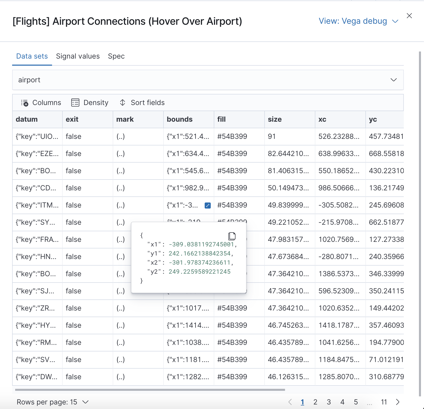
With the Vega debug view, you can inspect the Data sets and Signal Values runtime data.

The runtime data is read from the runtime scope.

×

To debug more complex specs, copy the Vega spec from the Spec tab and use the online Vega Editor to debug it.

Because of the dynamic nature of the data in Elasticsearch, it is hard to help you with Vega specs unless you can share a dataset. To do this, click Inspect, select the Vega debug view, then select Spec.

×

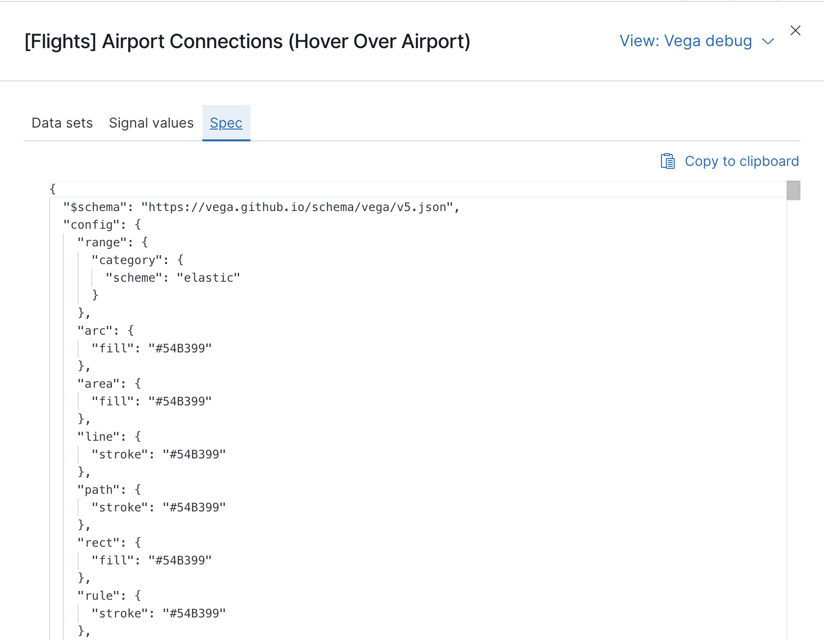
To copy the response, click Copy to clipboard. Paste the copied data to gist.github.com, possibly with a .json extension. Use the [raw] button, and share that when asking for help.

Kibana has extended the Vega expression language with these functions. These functions will trigger new data to be fetched, which by default will reset Vega signals. To keep signal values set restoreSignalValuesOnRefresh: true in the Vega config.

/**
  * @param {object} query Elastic Query DSL snippet, as used in the query DSL editor
  * @param {string} [index] as defined in Kibana, or default if missing
  * @param {string} Custom label of the filter shown in the filter bar
  */
kibanaAddFilter(query, index, alias)

/**
  * @param {object} query Elastic Query DSL snippet, as used in the query DSL editor
  * @param {string} [index] as defined in Kibana, or default if missing
  */
kibanaRemoveFilter(query, index)

kibanaRemoveAllFilters()

/**
  * Update dashboard time filter to the new values
  * @param {number|string|Date} start
  * @param {number|string|Date} end
  */
kibanaSetTimeFilter(start, end)
		

{
  config: {
    kibana: {
      // Placement of the Vega-defined signal bindings.
      // Can be `left`, `right`, `top`, or `bottom` (default).
      controlsLocation: top
      // Can be `vertical` or `horizontal` (default).
      controlsDirection: vertical
      // If true, hides most of Vega and Vega-Lite warnings
      hideWarnings: true
      // Vega renderer to use: `svg` or `canvas` (default)
      renderer: canvas
      // Defaults to 'false', restores Vega signal values on refresh
      restoreSignalValuesOnRefresh: false
    }
  }
}
		

To learn more about Vega and Vega-Lite, refer to the resources and examples.

The Vega Editor includes examples for Vega & Vega-Lite, but does not support any Kibana-specific features like Elasticsearch requests and interactive base maps.

• Tutorials
• Docs
• Examples

• Tutorials
• Docs
• Examples