Build area charts with Kibana
Area charts are line charts with the area below the line filled in with a certain color or texture. Area charts work with numeric metrics over the horizontal axis (typically time) and are ideal to display quantitative values over an interval or time period, to show trends for time series like traffic, CPU, revenue, or error rates.
You can build an area chart in Kibana in either of these ways:
To automate chart or dashboard creation, use the Dashboards and Visualizations APIs. To create dashboards from natural-language instructions, use Elastic Agent Builder or the Kibana dashboards agent skill.
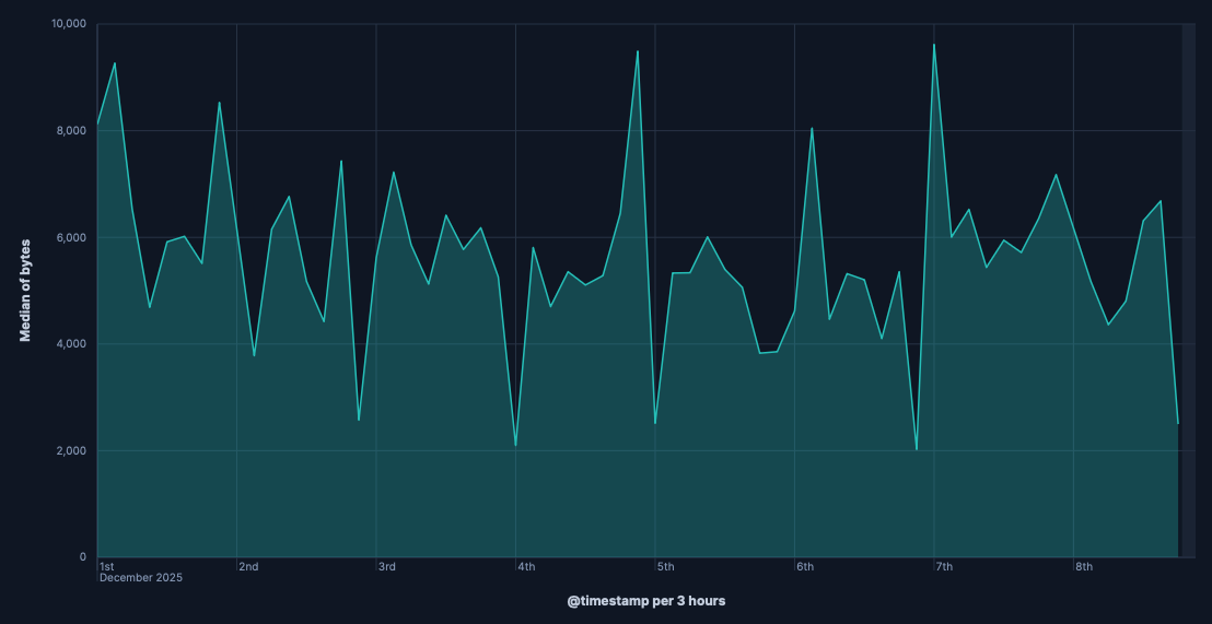
Before you start, make sure you have data indexed into Elasticsearch or install sample data. The point-and-click editor uses data views to access your Elasticsearch data. Data views are usually created automatically when you ingest data. You can also create one manually to select the data that you want.
To build an area chart:
-
Access Lens
Lens is Kibana's main visualization editor. You can access it:
- From a dashboard: On the Dashboards page, open or create the dashboard where you want to add the visualization, then add a new visualization.
- From the Visualize library page by creating a new visualization.
-
Set the visualization to Area
New visualizations often start as Bar charts.
Using the Visualization type dropdown, select Area.
-
Define the data to show
- Select the data view that contains your data.
- Drag a time field to the Horizontal axis and a numeric field to the Vertical axis. Kibana automatically selects an appropriate aggregation function compatible with the selected field.
Optionally:
- Add more numeric fields to create additional series, or drag a categorical field to the Breakdown settings to segment your data by a categorical field, and create multiple areas within the same chart.
- You can click the Add layer icon to integrate additional visualizations, annotations, or a reference line.
The chart preview updates to show filled areas plotted over time. Each area represents a series, with the filled region emphasizing the volume of data.
-
Save the chart
- If you accessed Lens from a dashboard, select Save and return to save the visualization and add it to that dashboard, or select Save to library to add the visualization to the Visualize library and be able to add it to other dashboards later.
- If you accessed Lens from the Visualize library, select Save. A menu opens and lets you add the visualization to a dashboard and to the Visualize library.
Before you start, make sure you have data indexed into Elasticsearch or install sample data. ES|QL queries the indices named in the query directly, so you do not need a data view. The columns returned by the query become available as chart dimensions. Refer to Visualizations using ES|QL queries to learn how to open the editor, shape the query result for a visualization, and save the visualization.
A time-series area chart needs a time-bucket column for its horizontal axis and a numeric metric column for the height of the filled area. In this query, WHERE applies the dashboard time range, BUCKET divides that range into 50 adaptive groups, and SUM returns one metric value for each group:
FROM kibana_sample_data_logs
| WHERE @timestamp <= ?_tend AND @timestamp > ?_tstart
| STATS total_bytes = SUM(bytes) BY time_bucket = BUCKET(@timestamp, 50, ?_tstart, ?_tend)
To build the chart:
- Create an ES|QL visualization and run the query.
- Set the visualization type to Area.
- Assign
time_bucketto the Horizontal axis andtotal_bytesto the Vertical axis. - Customize the chart appearance using the area chart settings.
- Select Apply and close.
The chart preview shows how the volume of transferred data changes over time.
After building the chart with the point-and-click editor or an ES|QL query, customize its appearance for your data and audience:
- Select the appropriate stack mode
- Use Stacked to show contribution to a whole, Percentage for normalized representation of values, or Unstacked when absolute trends matter more than composition. For a practical use case, check how to show composition with stacked and 100% stacked areas.
- Handle gaps and noise
- For sparse data, configure Missing values and Line interpolation to avoid misleading gaps or sharp edges. Refer to General layout settings.
- Use color purposefully
- Apply colors to highlight important data or patterns. Avoid using too many colors that might distract from the data. You can also assign consistent colors to key categories.
- Label clearly
- Provide a descriptive title and axis labels that clearly communicate what the chart shows. For example, mention the metric being visualized ("Average Response Time") and reference the time period when relevant ("Dec 8-16, 2025").
Refer to Area chart settings for all area chart configuration options. For panel sizing and layout guidance, refer to Organize dashboard panels.
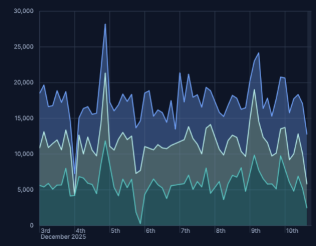
Use stacking to show how categories contribute to a total over time.
Create an area chart with a time-based Horizontal axis.
Break down the series by a categorical field, for example,
agent.keyword,response.keyword. You can set the area chart stack mode to:Stacked — Show cumulative totals and category contributions.
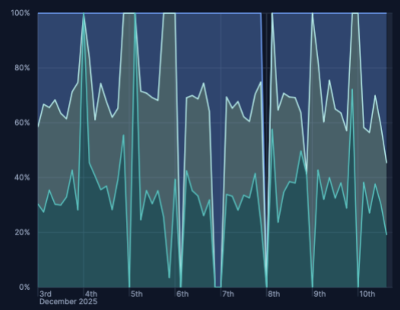
Percentage (100%) — Normalizes each timestamp to 100% to emphasize shares rather than magnitudes.
Optionally, in the Breakdown settings, you can set Rank by to specify the dimension the top values are ranked by.
In Area charts, you can enable time shift to compare different periods and identify deltas.
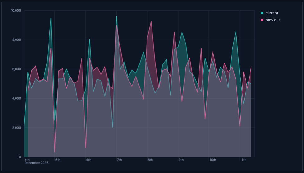
- Create an area chart with a time-based Horizontal axis and your main metric on Vertical axis, for example:
bytes. - Duplicate the layer:
-
Select Duplicate layer from the visualization editor. -
Open the contextual menu of the visualization editor and select Duplicate layer.
-
- From the duplicated layer settings, select the field defined as vertical axis to open its details. Expand its Advanced options and set Time shift to
1wor to the time value of your choice. Check Compare differences over time for more details. - Optionally, customize the appearance of the layer to adjust how it looks on the chart. When you duplicate a layer, Kibana automatically assigns a different Series color to the new layer. You can for example change this color, or adjust the layer's name and axis position. This name is used for the chart's legend.
You can also compute the relative change using a formula, for example:
(average(bytes) - average(bytes, shift='1w')) / average(bytes, shift='1w')
Customize your area chart to match the information you need and how you want it displayed.
- Data
-
- Functions:
- Top values: Show the most common values of a field.
- Field: Select the field to group by. You can add up to 4 fields to create multi-term groups. When multiple fields are selected, each group represents a unique combination of values across those fields. You can reorder the fields by dragging them to change their priority.
- Number of values: How many top values to display. The default number of values depends on your environment:
-
Defaults to 9. -
Defaults to 5 for the first Top values dimension added to the chart and 3 for each additional one.
-
- Rank by: Specifies the dimension the top values are ranked by. Available options:
- Count of records: Rank by the number of documents containing each value. This is the default when a metric is defined.
- Alphabetical: Rank by the term key alphabetically. This is the default when no metric is defined.
- Rarity: Find terms that appear in very few documents, using a rare terms aggregation. You can configure the Max doc count per term to set the maximum number of documents a term can appear in to be considered rare (default: 1, max: 100). Available for single-field terms only, and not for floating-point numeric fields (
float,double,half_float, andscaled_float). - Significance: Find statistically unusual terms compared to the overall data set, using a significant terms aggregation. Only available for
keywordfields and single-field terms. - Custom: Define a custom metric aggregation to rank by (for example, rank by the sum of a numeric field rather than by count).
- Rank direction: Ascending or descending order. Disabled when Rank by is set to Rarity or Significance.
Advanced settingsSeveral advanced options allow you to refine the behavior of the breakdown:
- Include documents without the selected field: Off by default.
- Group remaining values as "Other": On by default.
- Enable accuracy mode: This option improves results for high-cardinality data, but increases the load on the Elasticsearch cluster.
- Include values: Values from the dimension to always include, even if they aren't among the top values. You can enter exact values or a regular expression.
- Exclude values: Values from the dimension to always exclude. You can enter exact values or a regular expression.
- Date histogram: Group data into time-based buckets.
- Field: Select the date field to use for the time-based grouping.
Include empty rows: Include buckets that contain no matching documents. Existing saved visualizations keep their configured setting.
For new visualizations, this option is: - On by default for tables, line charts, and area charts
- Off by default for bar charts, heat maps, pie charts, treemap charts, mosaic charts, waffle charts, metric charts, and tag clouds
When you switch visualization or series type, Lens applies the default for the new type. If you switch back to the visualization type you saved, Lens restores the saved setting.
This option is on by default for all visualization types.
Bind to global time picker: Associate the selected field to the Lens or dashboard main time selector.
Minimum interval: Define the time interval for aggregating the data. For example,
30s,20m,24h,2d,1w,1MDrop partial intervals: Exclude incomplete intervals from the data. This option is off by default.
- Intervals: Create numeric ranges for continuous data by grouping a numeric field into buckets.
- Field: Select the numeric field to create intervals from.
- Intervals granularity: Use the slider to control how many intervals to create. Kibana divides the field into evenly spaced intervals (incremented by 10, 5, or 2) between the field's minimum and maximum values. The minimum granularity is 1, and the maximum is set by the
histogram:maxBarsadvanced setting. - Create custom ranges: Define your own ranges with specific lower and upper bounds and optional labels, instead of using the automatic granularity.
- Include empty rows: Include intervals that contain no matching documents. Existing saved visualizations keep their configured setting.
For new visualizations, this option is: - On by default for tables, line charts, and area charts
- Off by default for bar charts, heat maps, pie charts, treemap charts, mosaic charts, waffle charts, metric charts, and tag clouds
When you switch visualization or series type, Lens applies the default for the new type. If you switch back to the visualization type you saved, Lens restores the saved setting.
This option is on by default for all visualization types.
- Filters: Define custom KQL filters. Each filter creates one group from the documents that match its query.
- Top values: Show the most common values of a field.
- Functions:
- Appearance
- Name: By default, the chart uses the function or formula as title. It's a best practice to customize this with a meaningful title.
- Data
-
To represent the metrics or values you want to visualize, you can use quick functions like Average, Count, Percentile, Counter rate, or create custom calculations with formulas. Refer to Lens visualizations > Use formulas to perform math for examples.
Advanced settingsDepending on the data you defined, several options allow you to apply additional filtering to the data taken into account to compute the final value to show.
Based on the type of visualization you're creating, only some of the following options can be available:
- Normalize by unit: Normalize the metric values to show per unit of time.
- Filter by: Specify a query.
- Reduced time range: Reduce the time range specified on the dashboard's time filter by the specified duration.
- Time shift: Shift the time range by the specified duration. This is useful if the value should use a different time range than the one selected on the dashboard.
- Hide zero values: Don't show values equal to zero. This option is on by default.
- Appearance
-
Configure series-level options, including:
- Name: Customize the series label.
- Value format: Control how numeric values are displayed on your vertical axis and in tooltips.
- Series color: Determine the color of your data series in the visualization.
- Axis side: Determine which side of the chart the vertical axis appears on.
You can split your data by a categorical field to create multiple stacked or overlapping areas. You can specify the following options:
- Data
-
- Functions:
- Top values: Show the most common values of a field.
- Field: Select the field to group by. You can add up to 4 fields to create multi-term groups. When multiple fields are selected, each group represents a unique combination of values across those fields. You can reorder the fields by dragging them to change their priority.
- Number of values: How many top values to display. The default number of values depends on your environment:
-
Defaults to 9. -
Defaults to 5 for the first Top values dimension added to the chart and 3 for each additional one.
-
- Rank by: Specifies the dimension the top values are ranked by. Available options:
- Count of records: Rank by the number of documents containing each value. This is the default when a metric is defined.
- Alphabetical: Rank by the term key alphabetically. This is the default when no metric is defined.
- Rarity: Find terms that appear in very few documents, using a rare terms aggregation. You can configure the Max doc count per term to set the maximum number of documents a term can appear in to be considered rare (default: 1, max: 100). Available for single-field terms only, and not for floating-point numeric fields (
float,double,half_float, andscaled_float). - Significance: Find statistically unusual terms compared to the overall data set, using a significant terms aggregation. Only available for
keywordfields and single-field terms. - Custom: Define a custom metric aggregation to rank by (for example, rank by the sum of a numeric field rather than by count).
- Rank direction: Ascending or descending order. Disabled when Rank by is set to Rarity or Significance.
Advanced settingsSeveral advanced options allow you to refine the behavior of the breakdown:
- Include documents without the selected field: Off by default.
- Group remaining values as "Other": On by default.
- Enable accuracy mode: This option improves results for high-cardinality data, but increases the load on the Elasticsearch cluster.
- Include values: Values from the dimension to always include, even if they aren't among the top values. You can enter exact values or a regular expression.
- Exclude values: Values from the dimension to always exclude. You can enter exact values or a regular expression.
- Date histogram: Group data into time-based buckets.
- Field: Select the date field to use for the time-based grouping.
Include empty rows: Include buckets that contain no matching documents. Existing saved visualizations keep their configured setting.
For new visualizations, this option is: - On by default for tables, line charts, and area charts
- Off by default for bar charts, heat maps, pie charts, treemap charts, mosaic charts, waffle charts, metric charts, and tag clouds
When you switch visualization or series type, Lens applies the default for the new type. If you switch back to the visualization type you saved, Lens restores the saved setting.
This option is on by default for all visualization types.
Bind to global time picker: Associate the selected field to the Lens or dashboard main time selector.
Minimum interval: Define the time interval for aggregating the data. For example,
30s,20m,24h,2d,1w,1MDrop partial intervals: Exclude incomplete intervals from the data. This option is off by default.
- Intervals: Create numeric ranges for continuous data by grouping a numeric field into buckets.
- Field: Select the numeric field to create intervals from.
- Intervals granularity: Use the slider to control how many intervals to create. Kibana divides the field into evenly spaced intervals (incremented by 10, 5, or 2) between the field's minimum and maximum values. The minimum granularity is 1, and the maximum is set by the
histogram:maxBarsadvanced setting. - Create custom ranges: Define your own ranges with specific lower and upper bounds and optional labels, instead of using the automatic granularity.
- Include empty rows: Include intervals that contain no matching documents. Existing saved visualizations keep their configured setting.
For new visualizations, this option is: - On by default for tables, line charts, and area charts
- Off by default for bar charts, heat maps, pie charts, treemap charts, mosaic charts, waffle charts, metric charts, and tag clouds
When you switch visualization or series type, Lens applies the default for the new type. If you switch back to the visualization type you saved, Lens restores the saved setting.
This option is on by default for all visualization types.
- Filters: Define custom KQL filters. Each filter creates one group from the documents that match its query.
- Top values: Show the most common values of a field.
- Collapse by: Aggregate all metric values that share the same value for this dimension into a single number, removing it as an independent grouping. Available aggregation methods:
Sum,Min,Max, orAverage.
- Functions:
- Appearance
-
Allow you to customize how your breakdown data is displayed in line charts, including:
- Name: It's a best practice to customize this with a meaningful title.
- Color mapping: Determine how colors are assigned to your breakdown series.
When creating or editing a visualization, you can adjust the following settings.
Style
Adjust the visual appearance of your area chart to control how the data series are labeled and displayed alongside your chart. Click to open the Style panel.
- Appearance
- Allow you to customize the overall chart appearance:
- Area fill opacity: Control how transparent or opaque the colored area beneath the data line appears. The opacity value ranges from 0 to 1.
- Point visibility: Show or hide data points. Set to Auto by default: Points are visible unless the distance between them is too short.
- Line interpolation: Choose how to interpolate the line between data points from the available options: Straight (default), Smooth, and Step.
- Left axis
- Allow you to customize the Y-axis appearance.
- Axis Title. Show, hide or add a custom title.
- Gridlines. Show or hide gridlines.
- Tick labels. Show or hide tick labels.
- Orientation. Choose the tick labels orientation.
- Axis scale. Choose an axis scale type. Options include: Linear (default), Logarithmic, and Square root.
- Bounds. Use Bounds to set the minimum and maximum values for the Y-axis. Options include: Full, Data, and Custom
- Round to nice value. Axis labels can be rounded to more readable numbers.
- Bottom axis
- Allow you to customize the bottom axis appearance:
- Axis Title. Show, hide or add a custom title.
- Gridlines. Show/hide gridlines.
- Tick labels. Show/hide tick labels.
- Show partial data markers: indicate data points where Data collection is incomplete (the time bucket is still open and actively collecting events), or data may change (the values represented might increase as more data arrives).
- Show current time marker: Add a vertical line on your chart that represents the current time.
Missing values
Use Missing values to control how gaps appear in area and line charts. Missing values include empty buckets and metrics that return null because of their operation or data.
This setting is available when Include empty rows is enabled or when a metric produces a null bucket. For example, a moving average can produce null buckets.
This setting isn't available for percentage area charts or charts created from ES|QL queries.
Hide: Don't show gaps in the data.
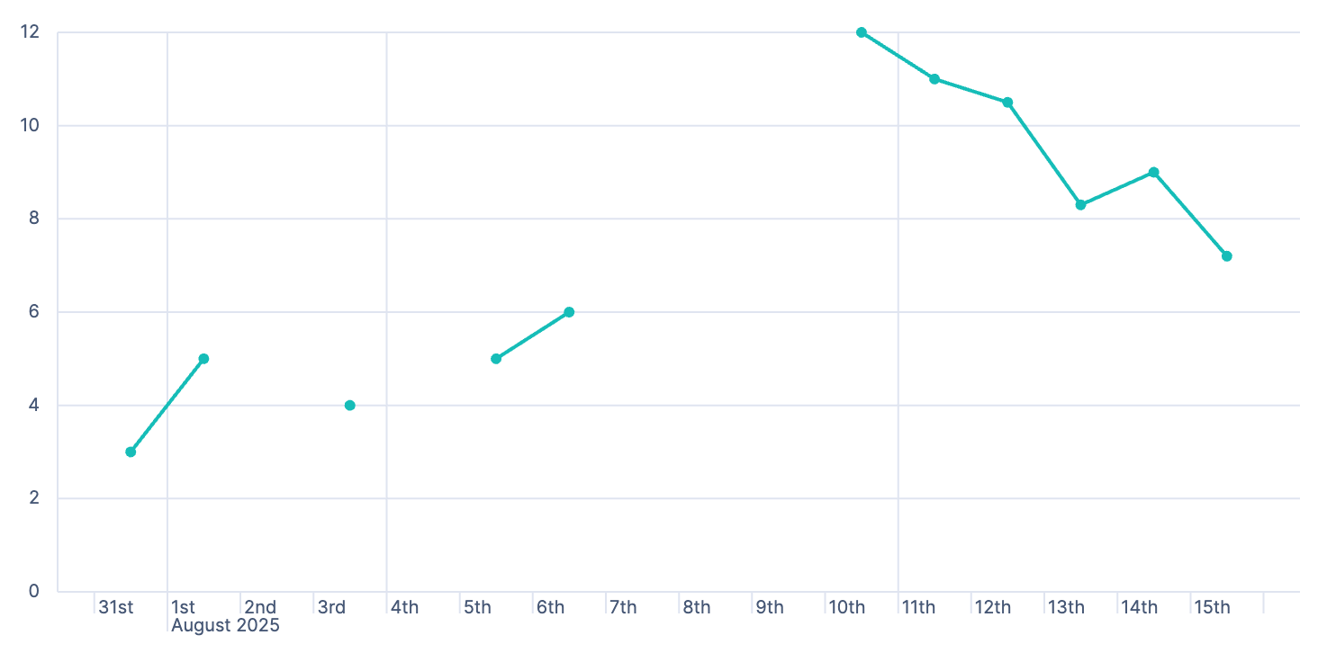
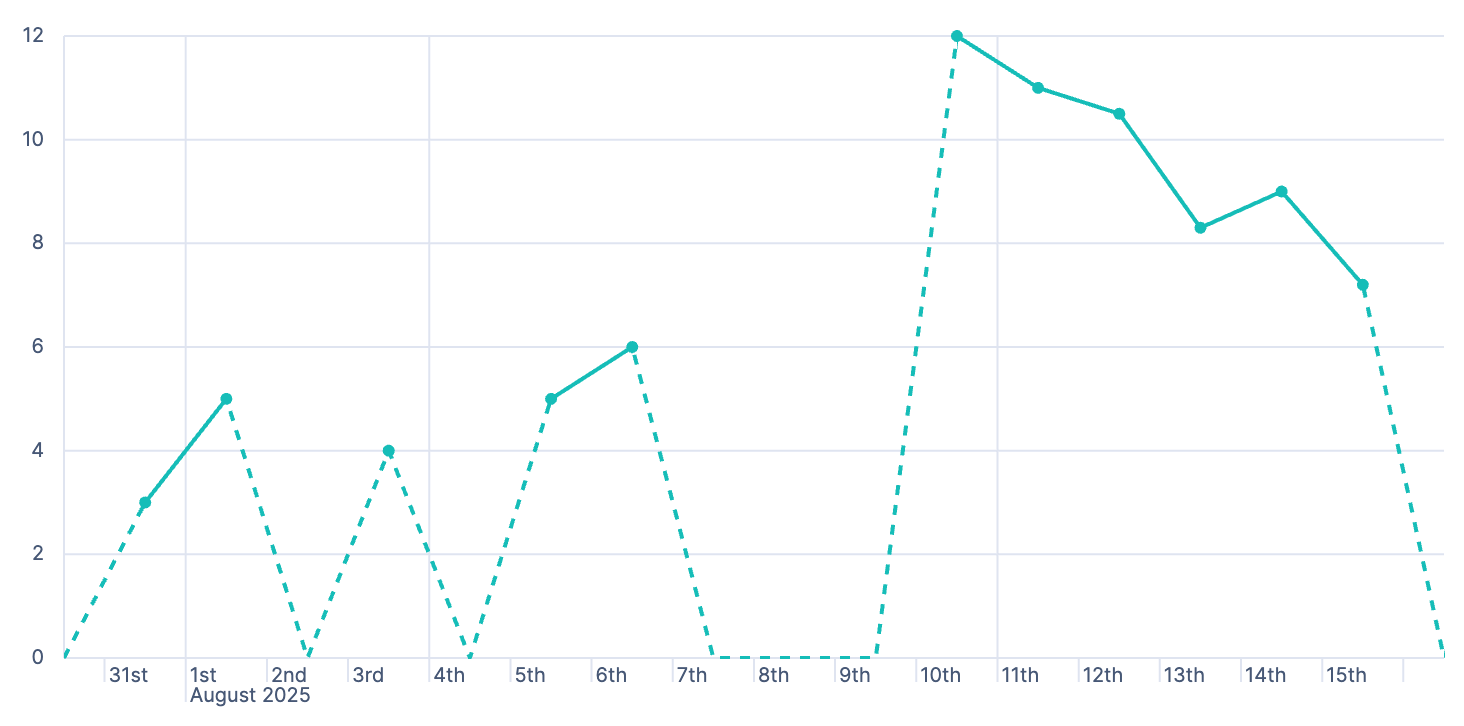
Zero: Connect the data points before and after each gap to zero.
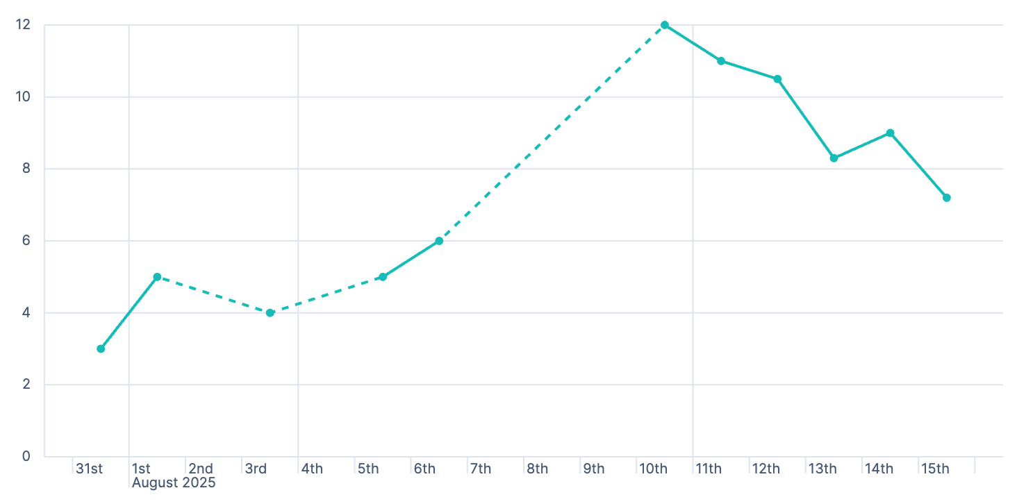
Linear: Connect the data points before and after each gap with a straight line.
Last: Fill each gap with a horizontal or vertical line from the last available data point.
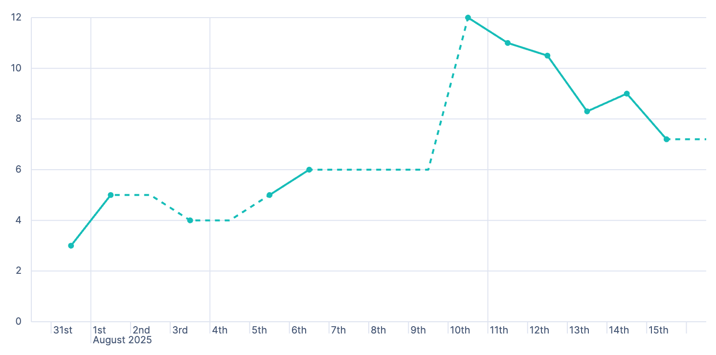
Next: Fill each gap with a horizontal or vertical line from the next available data point.
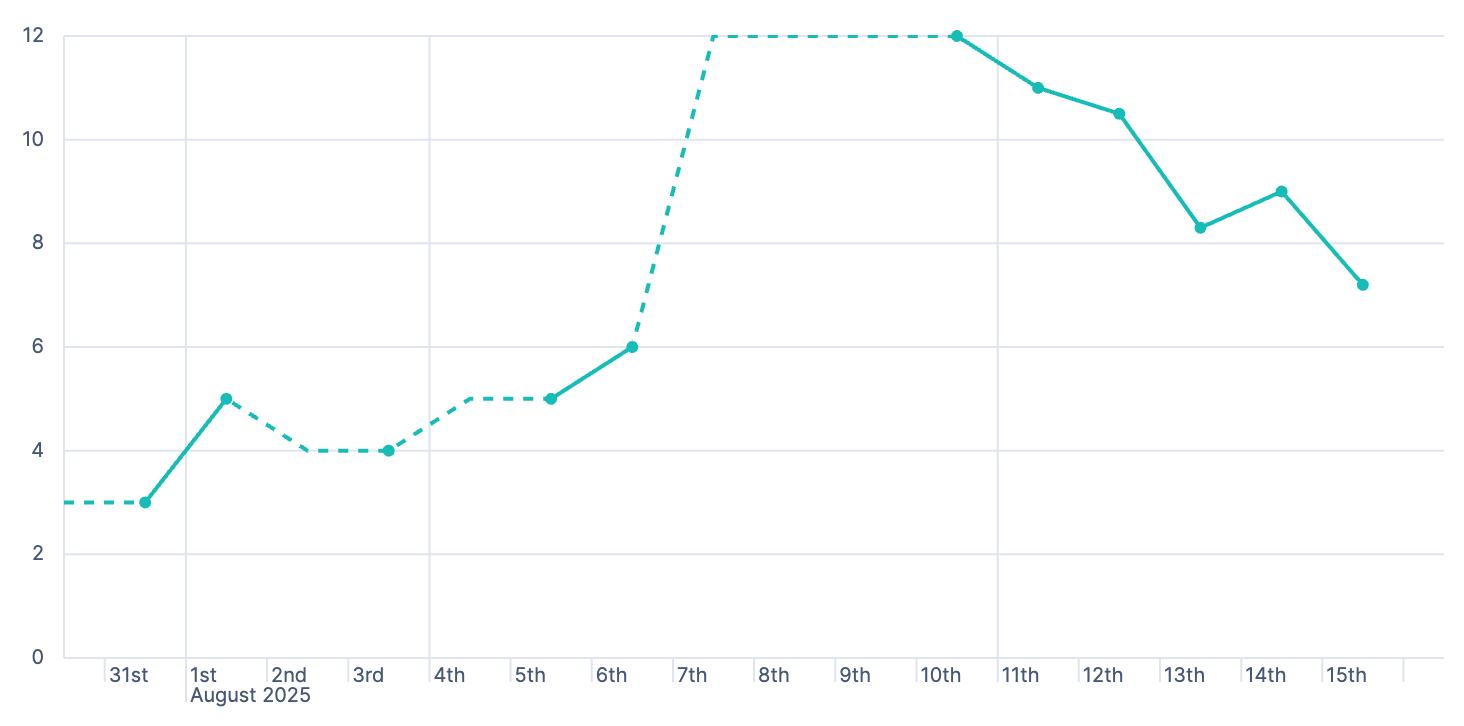
- End values
-
Choose how to extend a series to the edge of the chart:
- Hide: Don't extend the series.
- Zero: Extend the series as zero.
- Nearest: Extend the series using its first or last value.
- Show as dotted line
- Show the lines used to fill gaps as dotted lines.
Legend
You can customize the way the legend is displayed and the data it shows. Select  to open the Legend panel.
Use Visibility and Position to control where the legend appears.
For legends positioned outside the chart on the left or right, use Width to set the legend size.
- Layout
-
For legends positioned outside the chart at the top or bottom, choose how series labels are arranged:
- List: A compact layout that flows series labels to fit the available space. List is the default for new charts when the legend is at the top or bottom.
- Grid: A table-style layout that aligns series labels and statistics into rows and columns.
Existing visualizations retain their layout until you change it.
- Statistics
-
When every chart layer uses a non-categorical horizontal axis, such as a date, time, or numeric axis, select one or more statistics to show for each series:
- Average: Average of all values
- Median: Median value
- Minimum: Minimum value
- Maximum: Maximum value
- Range: Difference between the minimum and maximum values
- Last value: Last value
- Last non-null value: Last value that isn't null
- First value: First value
- First non-null value: First value that isn't null
- Difference: Difference between the first and last values
- Difference %: Percentage difference between the first and last values
- Sum: Sum of all values
- Count: Number of values
- Distinct count: Number of distinct values
- Variance: Variance of all values
- Std deviation: Standard deviation of all values
- Current or last value: Value of the data point under the pointer, or the last value when the pointer isn't over a data point
All statistics use the aggregated data points shown for the selected time range, not the original documents from Elasticsearch. After you select a statistic that uses the Grid layout, you can add a Series header above the legend entries.
- Label truncation
- For legends positioned inside the chart, outside on the side, or outside at the top or bottom with the Grid layout, choose whether to truncate long series labels and set the maximum number of lines for each label.
- Traffic by geographic region
-
Visualizing which geographic regions generate the most traffic:
- Horizontal axis:
@timestamp(Date histogram) - Vertical axis:
records - Breakdown:
geo.dest
- Horizontal axis:
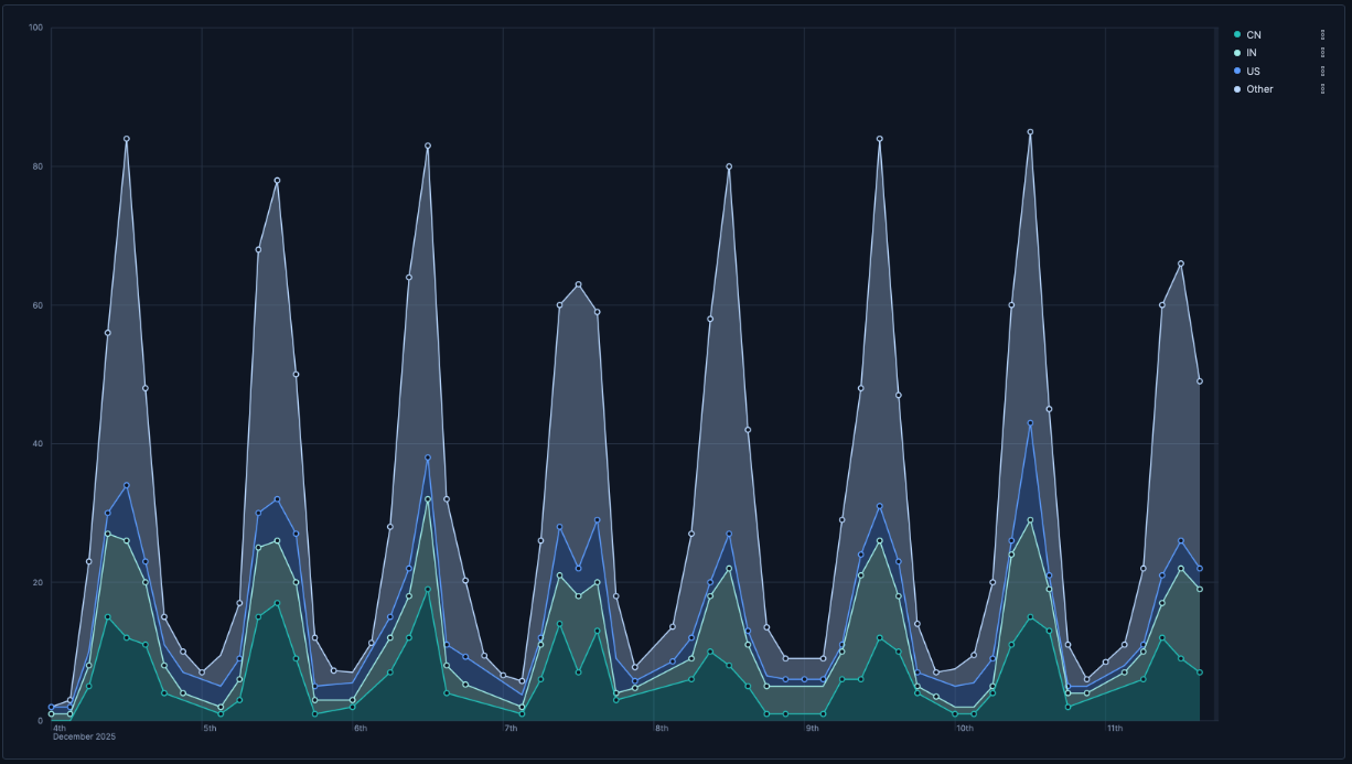
Send the following request to create a stacked area chart that shows record counts broken down by geographic destination.
These API request examples are kept up to date with the latest version of the APIs, so some fields might differ if you're using an earlier version. For a history of breaking changes, refer to the Kibana breaking changes or the Elastic Cloud Serverless breaking changes.
				POST kbn://api/visualizations
					{
  "type": "xy",
  "title": "Traffic by geographic region",
  "filters": [],
  "query": { "expression": "" },
  "legend": { "visibility": "auto", "placement": "outside", "position": "right" },
  "axis": {},
  "layers": [
    {
      "type": "area_stacked",
      "x": { "operation": "date_histogram", "field": "timestamp", "include_empty_rows": true },
      "y": [
        {
          "operation": "count",
          "empty_as_null": false,
          "label": "Records",
          "format": { "type": "number", "decimals": 0 },
          "filter": { "expression": "" }
        }
      ],
      "breakdown_by": {
        "operation": "terms",
        "fields": ["geo.dest"],
        "limit": 3,
        "other_bucket": { "include_documents_without_field": false },
        "rank_by": { "type": "metric", "metric_index": 0, "direction": "desc" },
        "aggregate_first": true
      },
      "data_source": {
        "type": "data_view_spec",
        "index_pattern": "kibana_sample_data_logs",
        "time_field": "timestamp"
      }
    }
  ],
  "styling": {
    "fitting": { "type": "none" },
    "areas": { "fill_opacity": 0.3 },
    "points": { "visibility": "visible" }
  }
}
- Uses
area_stackedto show each region's contribution to the total traffic. include_empty_rows: truefills time buckets with no data as zero rather than leaving gaps.- Shows only the top 3 geographic destinations.
other_bucketgroups all remaining destinations into an Other segment.aggregate_first: trueranks destinations globally across the full time range, ensuring the same top 3 appear consistently in every bucket.
curl -X POST "${KIBANA_URL}/api/visualizations" \
  -H "Authorization: ApiKey ${API_KEY}" \
  -H "kbn-xsrf: true" \
  -H "Content-Type: application/json" \
  -d '{
  "type": "xy",
  "title": "Traffic by geographic region",
  "filters": [],
  "query": { "expression": "" },
  "legend": { "visibility": "auto", "placement": "outside", "position": "right" },
  "axis": {},
  "layers": [
    {
      "type": "area_stacked",
      "x": { "operation": "date_histogram", "field": "timestamp", "include_empty_rows": true },
      "y": [
        {
          "operation": "count",
          "empty_as_null": false,
          "label": "Records",
          "format": { "type": "number", "decimals": 0 },
          "filter": { "expression": "" }
        }
      ],
      "breakdown_by": {
        "operation": "terms",
        "fields": ["geo.dest"],
        "limit": 3,
        "other_bucket": { "include_documents_without_field": false },
        "rank_by": { "type": "metric", "metric_index": 0, "direction": "desc" },
        "aggregate_first": true
      },
      "data_source": {
        "type": "data_view_spec",
        "index_pattern": "kibana_sample_data_logs",
        "time_field": "timestamp"
      }
    }
  ],
  "styling": {
    "fitting": { "type": "none" },
    "areas": { "fill_opacity": 0.3 },
    "points": { "visibility": "visible" }
  }
}'
- Uses
area_stackedto show each region's contribution to the total traffic. include_empty_rows: truefills time buckets with no data as zero rather than leaving gaps.- Shows only the top 3 geographic destinations.
other_bucketgroups all remaining destinations into an Other segment.aggregate_first: trueranks destinations globally across the full time range, ensuring the same top 3 appear consistently in every bucket.
For more information, refer to the Visualizations API.
Response code over time with annotations
Visualizing HTTP response codes over time, highlighting the proportion of success, client error, and server error responses, with annotations for key events:
- Horizontal axis:
@timestamp(Date histogram) - Vertical axis:
Count of records - Breakdown:
- Success/Redirection:
response.keyword >= 200 and response.keyword < 400 - Client Error:
response.keyword >= 400 and response.keyword < 500 - Server Error:
response.keyword >= 500
- Success/Redirection:
- Stacking:
Percentageto show the distribution relative to the total count at each point in time. - Annotation query:
tags:error AND tags:security
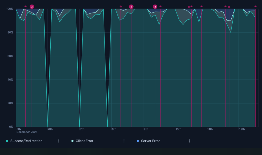
Send the following request to create a percentage area chart that shows the distribution of HTTP response codes over time.
These API request examples are kept up to date with the latest version of the APIs, so some fields might differ if you're using an earlier version. For a history of breaking changes, refer to the Kibana breaking changes or the Elastic Cloud Serverless breaking changes.
				POST kbn://api/visualizations
					{
  "type": "xy",
  "title": "Response code over time",
  "filters": [],
  "query": { "expression": "" },
  "legend": { "visibility": "auto", "placement": "outside", "position": "bottom", "layout": { "type": "list" } },
  "axis": {},
  "layers": [
    {
      "type": "area_percentage",
      "x": {
        "operation": "date_histogram",
        "field": "timestamp"
      },
      "y": [
        {
          "operation": "count",
          "empty_as_null": false,
          "label": "Count of records",
          "format": { "type": "number", "decimals": 2 },
          "filter": { "expression": "" }
        }
      ],
      "breakdown_by": {
        "operation": "filters",
        "filters": [
          {
            "filter": { "expression": "response.keyword >= 200 and response.keyword < 400" },
            "label": "Success/Redirection"
          },
          {
            "filter": { "expression": "response.keyword >= 400 and response.keyword < 500" },
            "label": "Client Error"
          },
          { "filter": { "expression": "response.keyword >= 500" }, "label": "Server Error" }
        ]
      },
      "data_source": {
        "type": "data_view_spec",
        "index_pattern": "kibana_sample_data_logs",
        "time_field": "timestamp"
      }
    },
    {
      "type": "annotations",
      "ignore_global_filters": true,
      "events": [
        {
          "type": "query",
          "label": "Event",
          "query": { "language": "kql", "expression": "tags:error AND tags:security" },
          "time_field": "timestamp",
          "color": { "type": "static", "color": "#ee72a6" },
          "visible": true,
          "icon": "asterisk"
        }
      ],
      "data_source": {
        "type": "data_view_spec",
        "index_pattern": "kibana_sample_data_logs",
        "time_field": "timestamp"
      }
    }
  ],
  "styling": {
    "fitting": { "type": "none" },
    "areas": { "fill_opacity": 0.3 }
  }
}
area_percentagenormalizes each time bucket to 100% so you see the proportion of each response class, not absolute counts.filtersbreakdown creates one area per KQL filter instead of splitting by field values.- The
annotationslayer marks events matchingtags:error AND tags:securityon the time axis with a pink asterisk.
curl -X POST "${KIBANA_URL}/api/visualizations" \
  -H "Authorization: ApiKey ${API_KEY}" \
  -H "kbn-xsrf: true" \
  -H "Content-Type: application/json" \
  -d '{
  "type": "xy",
  "title": "Response code over time",
  "filters": [],
  "query": { "expression": "" },
  "legend": { "visibility": "auto", "placement": "outside", "position": "bottom", "layout": { "type": "list" } },
  "axis": {},
  "layers": [
    {
      "type": "area_percentage",
      "x": {
        "operation": "date_histogram",
        "field": "timestamp"
      },
      "y": [
        {
          "operation": "count",
          "empty_as_null": false,
          "label": "Count of records",
          "format": { "type": "number", "decimals": 2 },
          "filter": { "expression": "" }
        }
      ],
      "breakdown_by": {
        "operation": "filters",
        "filters": [
          {
            "filter": { "expression": "response.keyword >= 200 and response.keyword < 400" },
            "label": "Success/Redirection"
          },
          {
            "filter": { "expression": "response.keyword >= 400 and response.keyword < 500" },
            "label": "Client Error"
          },
          { "filter": { "expression": "response.keyword >= 500" }, "label": "Server Error" }
        ]
      },
      "data_source": {
        "type": "data_view_spec",
        "index_pattern": "kibana_sample_data_logs",
        "time_field": "timestamp"
      }
    },
    {
      "type": "annotations",
      "ignore_global_filters": true,
      "events": [
        {
          "type": "query",
          "label": "Event",
          "query": { "language": "kql", "expression": "tags:error AND tags:security" },
          "time_field": "timestamp",
          "color": { "type": "static", "color": "#ee72a6" },
          "visible": true,
          "icon": "asterisk"
        }
      ],
      "data_source": {
        "type": "data_view_spec",
        "index_pattern": "kibana_sample_data_logs",
        "time_field": "timestamp"
      }
    }
  ],
  "styling": {
    "fitting": { "type": "none" },
    "areas": { "fill_opacity": 0.3 }
  }
}'
area_percentagenormalizes each time bucket to 100% so you see the proportion of each response class, not absolute counts.filtersbreakdown creates one area per KQL filter instead of splitting by field values.- The
annotationslayer marks events matchingtags:error AND tags:securityon the time axis with a pink asterisk.
For more information, refer to the Visualizations API.