Lens visualizations using ES|QL queries
Creating visualizations using an ES|QL query is particularly useful when you need to:
- Query data across multiple indices without a pre-configured data view
- Apply complex filtering, transforms, or custom calculations in a single query
- Prototype a visualization directly from an ES|QL query in Discover
For less advanced aggregations on a known index, the point-and-click mode is a good alternative.
You can add ES|QL visualizations to a dashboard directly from queries in Discover, or you can start from a dashboard.
If your visualization's query uses exactly one STATS command, dashboard users can turn on
Fast mode to get faster, estimated results for it. Refer to Use ES|QL in Kibana > Get faster results with approximate STATS.
In Discover, an ES|QL query shows a visualization when the query transforms the results, for example, with STATS or KEEP, or when the results have a time field. The time field is @timestamp, or the field that the query compares with the ?_tstart and ?_tend parameters. The query determines the visualization type, such as a histogram or a bar chart. To change the visualization type and display options, select
Edit visualization.
To add the visualization to an existing or a new dashboard, select Save visualization to dashboard. In earlier versions, select Save visualization.
Add a new panel from your dashboard.
-
Select Add in the application menu and, if required, New panel. -
Select Add panel in the application menu.
TipIf you haven't created a data view and you don't have a dashboard yet, the Dashboards page offers you the possibility to Try ES|QL right away. By selecting this option, a dashboard is created with an ES|QL visualization that you can interact with and configure using ES|QL.
-
Select Create visualization (query) (Visualization (query) or ES|QL under Visualizations in earlier versions).
An ES|QL editor appears and lets you configure your query and its associated visualization. The Suggestions panel can help you find alternative ways to configure the visualization.
TipCheck the ES|QL reference to get familiar with the syntax and optimize your query.
When editing your query or its configuration, run the query to update the preview of the visualization.
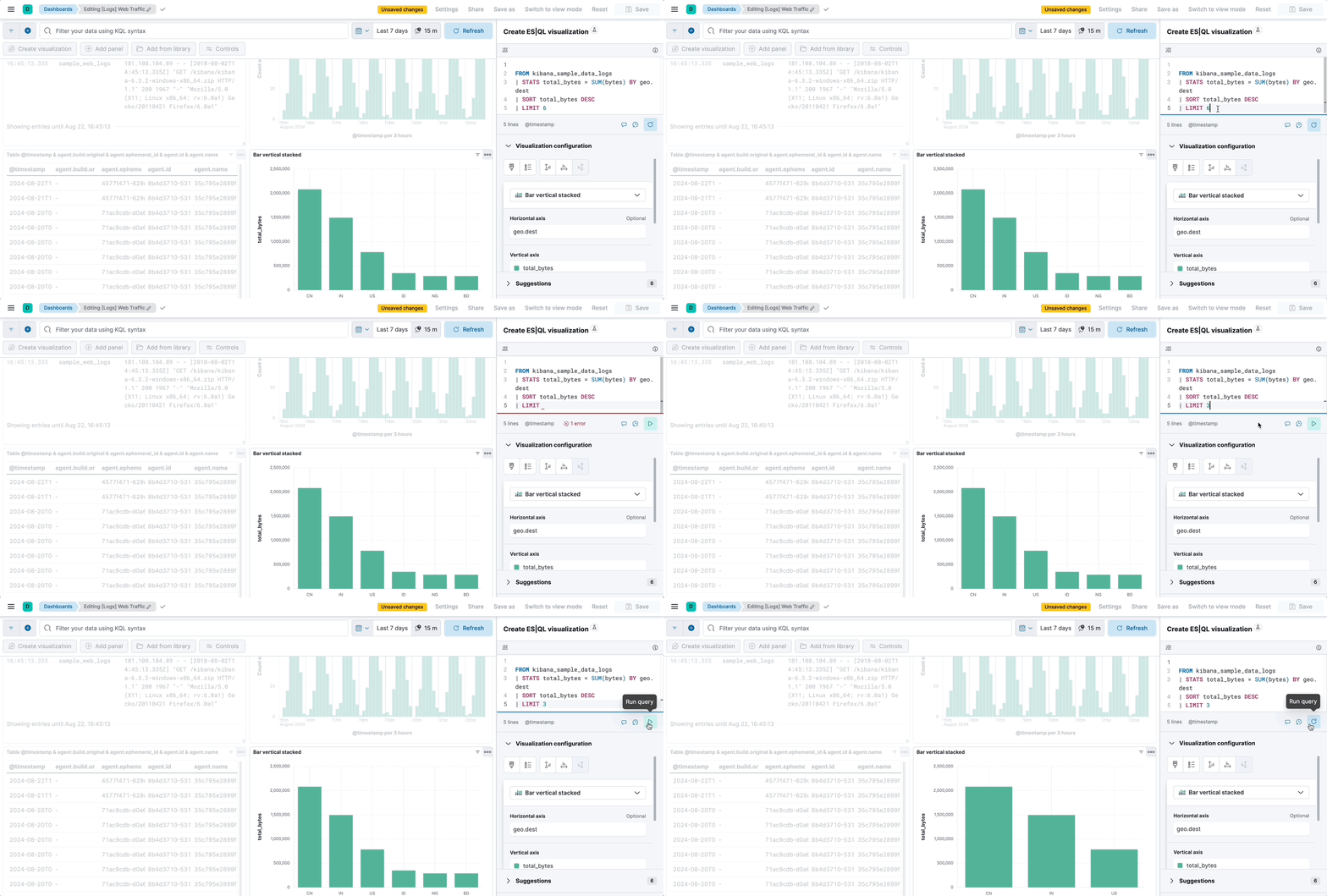 Note
When you edit the query and run it again, the visualization configuration persists as long as it is compatible with the query changes. Refer to Lens visualizations using ES|QL queries > Chart configuration persistence over ES|QL query update for more details.
You can bind controls to your ES|QL visualizations in dashboards by creating ES|QL controls.
Select Apply and close to save the visualization to the dashboard.
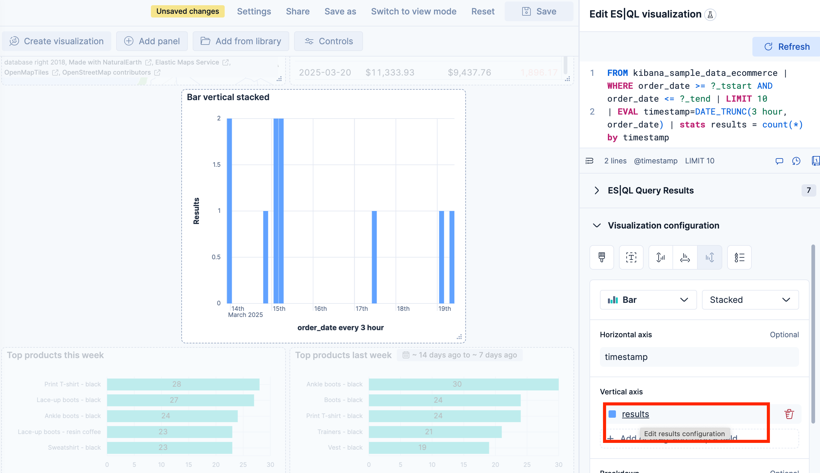
When editing an ES|QL visualization, you can customize the appearance of the chart. To do that:
Click one of the fields representing an axis of the chart to open its details.
Define the appearance of your choice from the available options.
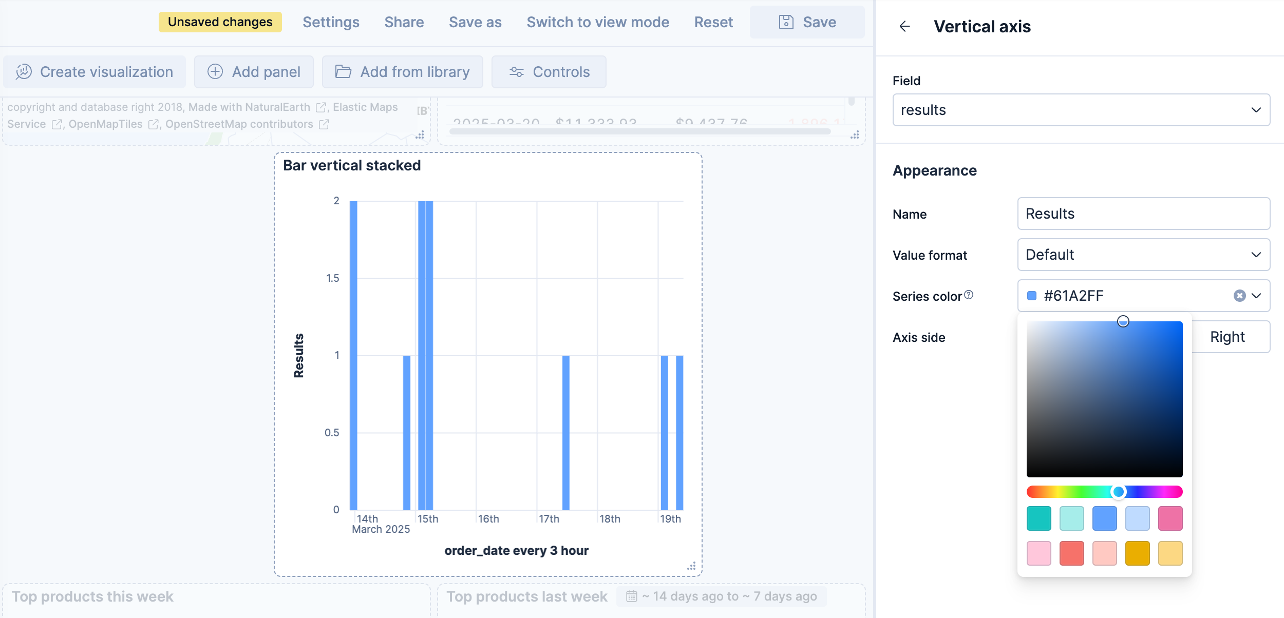
Return to the previous menu, then Apply and close the configuration to save your changes.
On bar, line, and area charts built from an ES|QL query, the Breakdown dimension can hold more than one field at the same time. Each unique combination of values is rendered as its own series, with the values joined by a › separator in the legend.
When the query groups a metric by more than one field, Kibana places the first field on the Horizontal axis and the remaining fields in the Breakdown dimension. For example, the following query counts web log events over time, broken down by host and file extension:
FROM kibana_sample_data_logs
| WHERE extension.keyword != ""
| STATS count(*) BY BUCKET(@timestamp, 100, ?_tstart, ?_tend), host.keyword, extension.keyword
In the resulting chart, the time buckets are placed on the Horizontal axis, while host.keyword and extension.keyword are combined in the Breakdown dimension. Each legend entry represents a unique combination, such as artifacts.elastic.co › deb or artifacts.elastic.co › gz.
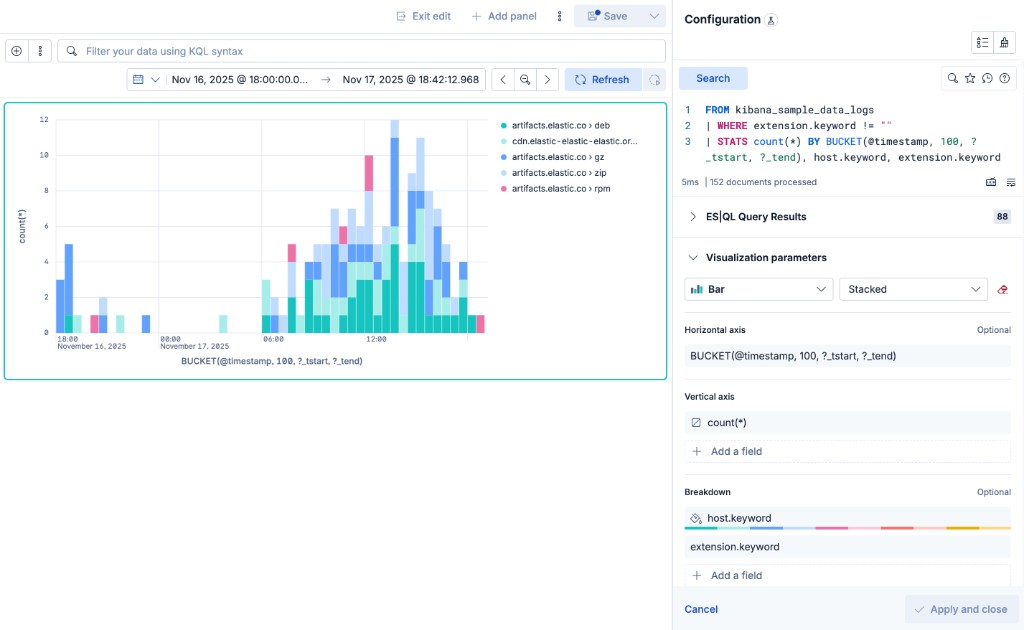
To add another field to the breakdown, select Add a field under Breakdown and choose a column from your query. You can also drag the fields inside the Breakdown dimension to change the order in which their values appear in the combined label.
When you create an ES|QL visualization from a dashboard, you can combine the results of several queries on one chart by giving each query its own layer. Layers can also hold annotations and reference lines, which mark events and thresholds on top of your data.
Every ES|QL data layer has its own query and its own dimensions, so you can change one query without touching the others. To split the results of a single query into several series instead, use the Breakdown dimension.
Layers are available on bar, line, and area charts. Other chart types, such as pie or metric, use a single query.
A chart can combine these layer types:
- Visualization: The results of its own query.
- Annotations: An event or a period, such as a deployment, marked on a time axis.
- Reference lines: A threshold, such as a target or a budget, drawn across the chart.
To add a layer, select Add layer in the editor, then select the type of layer. The new layer opens in its own tab.
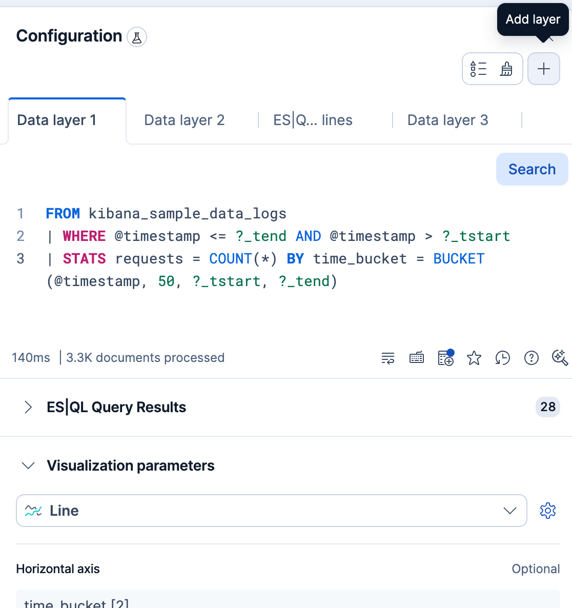
To compare two sets of results on one chart, add a layer with its own query:
- Select Add layer → Visualization.
- If you're asked, select the chart type for the layer. Each layer can use a different type, for example a line over bars.
- In the new layer's tab, enter the query and run it.
- Assign the column that holds time to the Horizontal axis and the column that holds the values to the Vertical axis.
Before you look at the chart, make sure both dimensions have a column. If the Horizontal axis of a layer is empty, the values of that layer don't follow time and stack at a single position. To line the layers up in time, group every query by the same time buckets and assign that column to the Horizontal axis of each layer.
If you edit a layer's query and its results no longer contain a compatible column for every dimension of that layer, Kibana rejects the query and shows an error. Remove the incompatible dimensions, then run the query again.
Example: Compare server and client errors
Start from the stacked bar chart of web log events.
Add a layer for the events that returned a server error (response codes that start with 5). If you're asked for a chart type, select Line. Use this query:
FROM kibana_sample_data_logs
| WHERE @timestamp <= ?_tend AND @timestamp > ?_tstart AND response.keyword LIKE "5*" AND extension.keyword != ""
| STATS server_errors = COUNT(*) BY time_bucket = BUCKET(@timestamp, 100, ?_tstart, ?_tend)
In this layer, assign
time_bucketto the Horizontal axis andserver_errorsto the Vertical axis.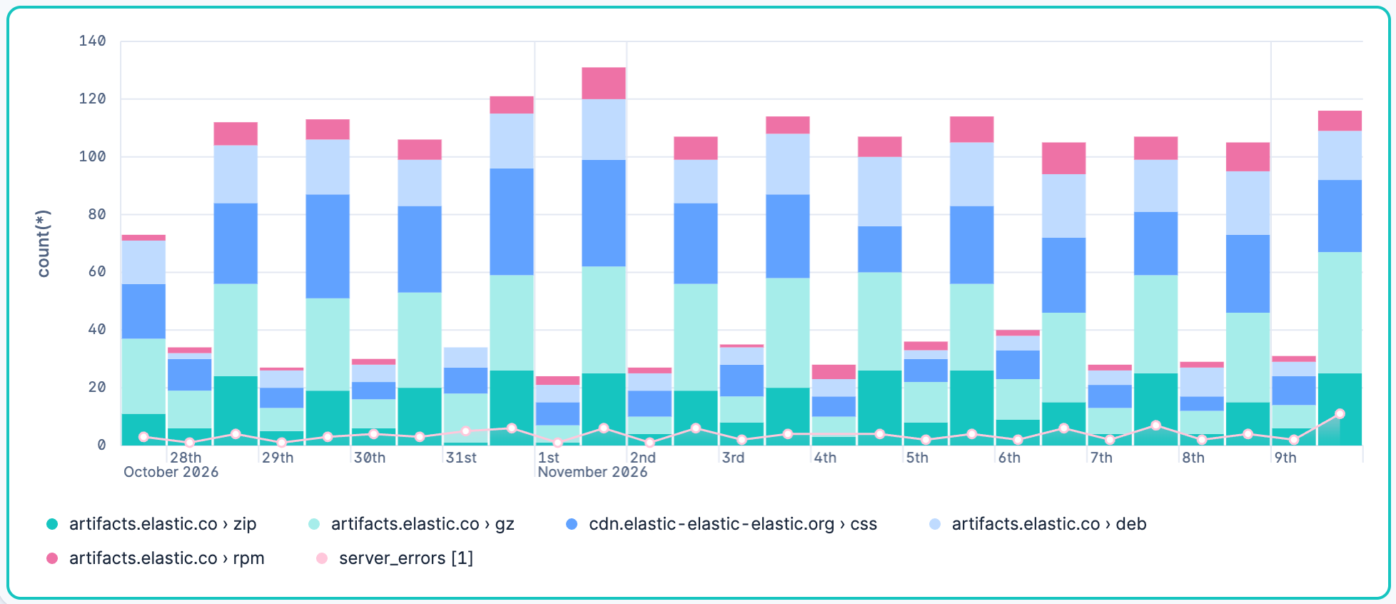
Add a third layer for the events that returned a client error (response codes that start with 4). Select Line again if you're asked for a chart type. Use this query:
FROM kibana_sample_data_logs
| WHERE @timestamp <= ?_tend AND @timestamp > ?_tstart AND response.keyword LIKE "4*" AND extension.keyword != ""
| STATS client_errors = COUNT(*) BY time_bucket = BUCKET(@timestamp, 100, ?_tstart, ?_tend)
In this layer, assign
time_bucketto the Horizontal axis andclient_errorsto the Vertical axis.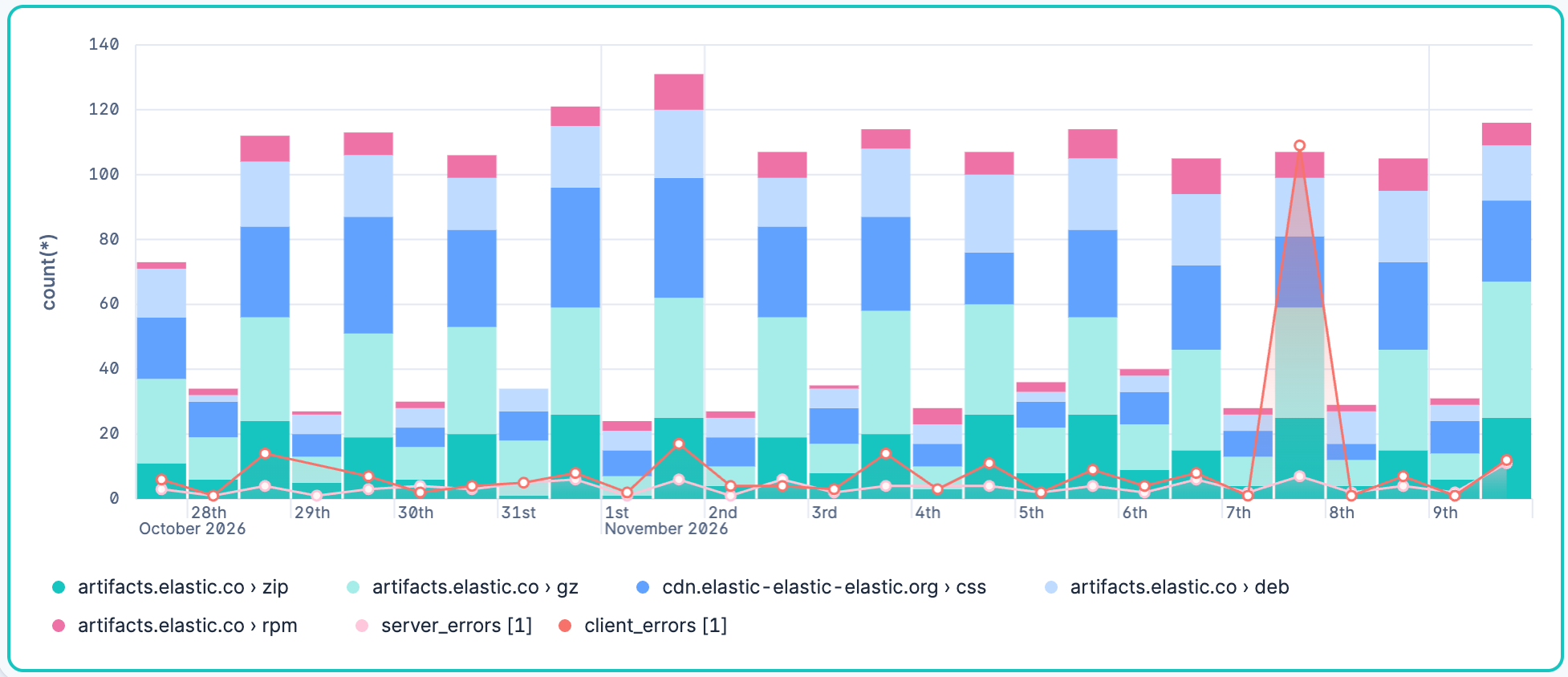
Annotations mark an event or a period on a time chart, such as a deployment or an outage. The chart needs a time axis, so Annotations stays unavailable until the horizontal axis shows time.
In the chart example that compares server and client errors of the previous section, the client errors spike on one day. To mark the outage behind that spike:
- Select Add layer → Annotations. Kibana creates an annotation immediately.
- Turn on Apply as range, then set From and To to the start and end of the outage.
- In Name, enter a label for the annotation, such as
eu-west-36 outage.
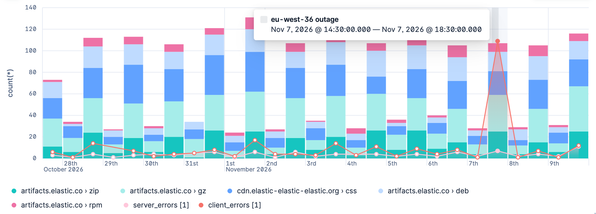
To mark a single moment instead, such as a deployment, leave Apply as range off and set Annotation date.
If you're used to adding annotations to visualizations created using the point-and-click editor, annotations on ES|QL visualizations work differently. You place each annotation yourself, by date or by date range. You can't base an annotation on a query or reuse one from the annotation library.
A reference line shows a threshold, such as a target or a budget, so you can see at a glance where your data crosses it.
On ES|QL visualizations, you can define a reference line in the following ways:
With a fixed value: Draw the line at a number that you choose.
- Select Add layer → Reference lines.
- If you're asked for a source, select Static reference lines.
- Set the value where you want the line to appear.
With a value from an ES|QL query: Calculate the threshold from your data, for example an average. - Select Add layer → Reference lines → ES|QL reference lines.
- Enter a query that returns the threshold in its first row, then run it.
- Select the column that holds the value for the line as the Vertical axis.
The line uses the first row of the results, and the column must contain a number. If the query returns more than one row, Kibana uses the first row and shows a warning.
The chart in the previous examples groups web log events into time buckets. To draw a line at the average number of events across those buckets, use this query. It counts the events in each time bucket, as the chart does, then averages the counts:
FROM kibana_sample_data_logs
| WHERE @timestamp <= ?_tend AND @timestamp > ?_tstart AND extension.keyword != ""
| STATS requests = COUNT(*) BY time_bucket = BUCKET(@timestamp, 100, ?_tstart, ?_tend)
| STATS average_requests = AVG(requests)
For this query, select
average_requestsas the Vertical axis.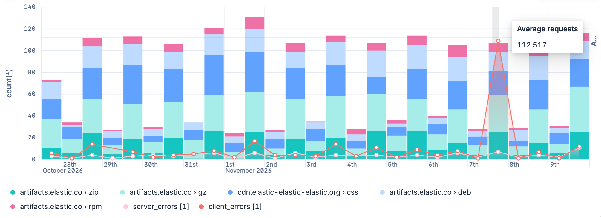
The Suggestions panel is hidden while the chart has more than one layer, because applying a suggestion would replace the other layers.
When you edit the ES|QL query and run it again, the visualization configuration persists as you defined it as long as it is compatible with the query changes.
The chart configuration resets or follows automatic suggestions when:
-
You manually select a different chart type incompatible with the one previously selected. -
You create a new chart and haven't edited the visualization's options yet. - The query changes significantly and no longer returns compatible columns.
When cross-project search is enabled and you have linked projects, your ES|QL visualization queries data based on the current cross-project search scope.
To target specific projects from within the query, add SET project_routing at the beginning of your ES|QL query. When you do this, the visualization panel displays a Custom CPS scope badge on the dashboard, indicating that it uses a different scope than the CPS scope selector. Refer to View data from multiple projects for details.
An ES|QL query returns a table. When you use the result to build a visualization, each returned column is available as a chart dimension. Shape the query result to provide the dimensions required by the chart:
| Result column | How to produce it | Common uses |
|---|---|---|
| Grouping column | Return a source column, group values with a BY clause, or derive a column with EVAL. |
Categories, rows, regions, series, and non-time axes |
| Time-bucket column | Group a time field with BUCKET or DATE_TRUNC. |
The horizontal axis of a time-series chart |
| Numeric metric column | Calculate a value with a STATS aggregation such as COUNT, SUM, or AVG. |
Plotted values, sizes, color intensity, metrics, and gauges |
The chart type determines the combination of columns you need. Open a page from the visualization types list to find an ES|QL query pattern and learn how to assign its result columns to the chart dimensions.
A time series chart plots a metric over time. The query must return a time-bucket column for the Horizontal axis and a numeric metric column for the Vertical axis.
In this query, WHERE applies the dashboard time range, BUCKET divides that range into 50 groups, and COUNT returns one value for each group:
FROM kibana_sample_data_logs
| WHERE @timestamp <= ?_tend AND @timestamp > ?_tstart
| STATS requests = COUNT(*) BY time_bucket = BUCKET(@timestamp, 50, ?_tstart, ?_tend)
If your time field isn't named @timestamp, replace @timestamp with that field in both WHERE and BUCKET. Refer to Use ES|QL in Kibana > Custom time parameters.
To build the chart:
- Create an ES|QL visualization and run the query.
- Set the visualization type to a chart type compatible with time series, typically Line, Area, or Bar.
- Assign
time_bucketto the Horizontal axis andrequeststo the Vertical axis. - Select Apply and close.
The chart preview shows how the request count changes over time.
For more query patterns and chart settings, refer to Build a line chart with an ES|QL query and Build an area chart with an ES|QL query.
To compare the current period with a previous period of the same duration, compute both windows in one STATS command. Use a per-aggregation WHERE filter for each window.
This example uses the Kibana sample web logs. It compares the last 7 days with the 7 days before that, per host. Add that data set if you don't have it yet. Sample data timestamps are relative to when you installed the data set.
To create the visualization:
Open a dashboard and add a new ES|QL visualization:
-
Select Add in the application menu, then select Create visualization (query) (Visualization (query) or New panel → ES|QL under Visualizations in earlier versions). -
Select Add panel in the application menu, then select ES|QL.
-
Set the time filter to the last 15 days so both 7-day windows have data.
Enter the following query:
FROM kibana_sample_data_logs | EVAL current_start = ?_tend - 7 days, previous_start = ?_tend - 14 days | STATS current_count = COUNT(*) WHERE @timestamp >= current_start AND @timestamp <= ?_tend, previous_count = COUNT(*) WHERE @timestamp >= previous_start AND @timestamp < current_start BY host.keyword | EVAL pct_diff = CASE( previous_count > 0, ROUND(100.0 * TO_DOUBLE(current_count - previous_count) / previous_count, 1), null ) | SORT ABS(pct_diff) DESC- Bound both windows from the end of the time filter.
?_tendstays in sync with the dashboard time filter. - Count events in each window in a single pass. Refer to
STATSwithWHERE. - Compute the percent change.
CASEreturnsnullwhen the previous window has no events.
- Bound both windows from the end of the time filter.
Run the query. A visualization appears with one row per host. If Kibana suggests a different visualization type, select Table from the visualization type dropdown.
Select Apply and close to save the visualization to your dashboard.
To use your own data, change the FROM source and the BY grouping field. If your time field isn't @timestamp, replace @timestamp in the STATS filters. To apply the dashboard time filter to a custom time field, add a WHERE clause with ?_tstart and ?_tend. Refer to Filter by time.
To compare a different duration or offset, change the two EVAL time spans. For the last hour versus the same hour a week ago, set current_start to ?_tend - 1 hour and previous_start to ?_tend - 7 days - 1 hour. Set the time filter to cover both windows.
To set Time shift in the point-and-click editor, refer to Compare differences over time.
ES|QL visualizations support the following drilldown types:
- Dashboard drilldowns: Open another dashboard from a data point.
- URL drilldowns: Open an external URL from a data point.
-
Discover drilldowns: Open Discover from a data point. Dashboard filters and the dashboard KQL or Lucene query are translated into the panel's ES|QL query, so the same context applies.
Drilldowns are compatible only with indexed fields. Fields created at query time are not supported. Refer to Values that cannot open a drilldown.
By default, an ES|QL visualization applies the filters and the KQL or Lucene query set at the dashboard level. To force a layer to run its query without these filters:
- Select the Settings icon on the layer header.
- Turn off Use global filters.
This option covers the dashboard's filter pills and the query from the search bar. The dashboard time range is a separate control that always applies, whether or not the option is turned on.
Once you've created an ES|QL panel, you can create an Elasticsearch threshold rule directly from the visualization panel, based on the data it displays. When you do this, the rule query is automatically generated and either describes the data and sets a specific threshold, or describes the data without setting a specific threshold.
Elastic Security rule types are not supported.
To create a rule with the threshold pre-specified:
- Right-click a data point in the visualization and click Add alert rule. This opens the Create rule flyout. The generated query will define a threshold that corresponds to the data point you selected.
- Configure your Elasticsearch rule.
To create a rule without the threshold pre-specified:
- Open the More actions (three dots) menu in the upper right of the panel and select Add alert rule. This opens the Create rule flyout. The generated query will define a threshold that corresponds to the data point you selected.
- Configure your Elasticsearch rule.
ES|QL query results can include emoji characters, which means you can use them in your ES|QL visualizations. Combined with EVAL and CASE functions, this opens up options like mapping values to colored status indicators (🟢, 🟠, 🔴), adding visual labels, or highlighting specific categories.
This example uses the Kibana sample web logs data to build a status table that shows the success rate per host, with a colored status indicator.
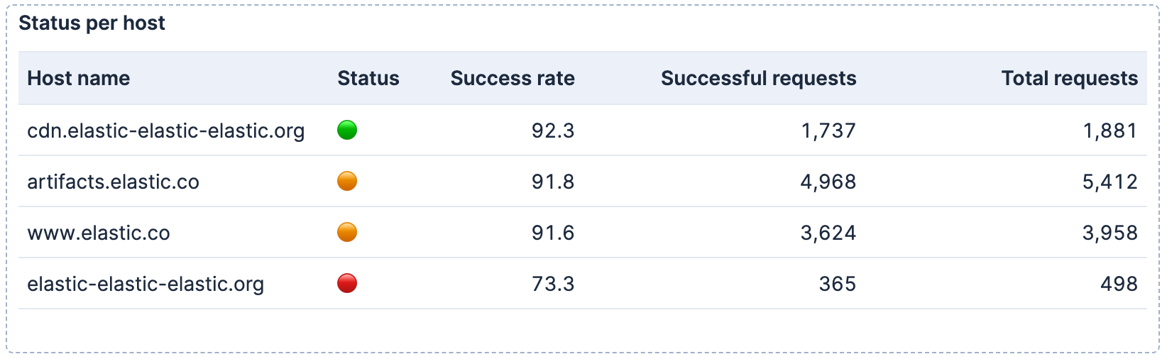
Because they're part of the query results, you can use them in any visualization type that displays text fields, such as bar charts with emoji labels or metric panels with status indicators.
Before you begin, ensure you have the sample web logs data installed. In Kibana, go to Integrations and search for Sample data. On the Sample data page, add Sample web logs.
To create the visualization:
Open a dashboard and add a new ES|QL visualization:
-
Select Add in the application menu, then select Create visualization (query) (Visualization (query) or New panel → ES|QL under Visualizations in earlier versions). -
Select Add panel in the application menu, then select ES|QL.
-
Enter the following query:
FROM kibana_sample_data_logs | EVAL is_success = CASE(response >= "200" AND response < "300", 1, 0) | STATS total_requests = COUNT(*), successful_requests = SUM(is_success) BY host.keyword | EVAL success_rate = ROUND(successful_requests * 100.0 / total_requests, 1) | EVAL status = CASE( success_rate >= 92, "🟢", success_rate >= 90, "🟠", "🔴" ) | KEEP host.keyword, status, success_rate, successful_requests, total_requests | SORT success_rate DESC- Create a binary flag: 1 for successful responses (2xx), 0 otherwise.
- Group by host and use
SUMto count successes. - Calculate the success rate as a percentage.
- Map the success rate to emoji indicators based on thresholds.
- Select and order the columns for the table output.
Run the query. A visualization appears with one row per host and an emoji status column. If Kibana suggests a different visualization type, select Table from the visualization type dropdown.
Optionally, configure the table appearance in the visualization settings:
- To reorder columns, rearrange the metrics in the Metrics section.
- To rename a column, select the metric and update its Name in the appearance options.
Select Apply and close to save the visualization to your dashboard.
Optionally, once the panel is saved, select the panel title to give it a meaningful name like
Status per host.
Once you have your visualization working, you can add controls to filter by host or time range, use LOOKUP JOIN to enrich your data with metadata from other indices, or create alerts based on the same query to get notified when status changes.